

![[*]](http://sepwww.stanford.edu/latex2html/prev_gr.gif)


![[*]](http://sepwww.stanford.edu/latex2html/foot_motif.gif)
ABSTRACTTime-lapse 3-D seismic monitoring of subsurface rock property changes incurred during reservoir fluid-flow processes is an emerging new diagnostic technology for optimizing hydrocarbon production. I discuss the physical theory relevant for three-phase fluid flow in a producing oil reservoir, and rock physics transformations of fluid-flow pressure, temperature and pore-fluid saturation values to seismic P-wave and S-wave velocity. I link fluid-flow physical parameters to seismic reflection data amplitudes and traveltimes through elastic wave equation modeling and imaging theory. I demonstrate with synthetic and field data examples that changes in fluid flow can be monitored and imaged from repeated seismic surveys acquired at varying production calendar times. |
INTRODUCTION Hydrocarbon reservoirs are increasingly recognized as spatially heterogeneous entities, in terms of pore-fluid content, pore-fluid saturation, porosity, permeability, lithology, and structural control. Knowledge of these reservoir parameters and their spatial variation is critical in the evaluation of the total volume of hydrocarbon reserves in place, in understanding and predicting physical processes in the reservoir such as fluid flow and heat transfer, and in projecting and monitoring reservoir fluid production and recovery as a function of time. A new diagnostic role for seismic has recently been proposed in which several repeat 3-D seismic surveys are acquired in time-lapse mode to monitor reservoir production fluid-flow processes, e.g, Nur . This 4-D monitoring concept offers a method for better characterization of reservoir complexity by monitoring the flow of fluids with time in a producing reservoir.
In this paper, I attempt to link fluid-flow physics, rock physics,
and the physics of seismic wave-theoretic modeling and imaging.
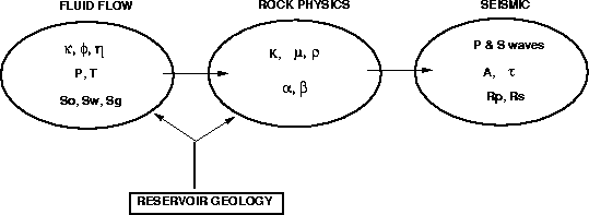
Figure ![[*]](http://sepwww.stanford.edu/latex2html/cross_ref_motif.gif) schematically shows how these three disciplines
are coupled in the seismic fluid-flow monitoring problem, and how
the critical physical parameters in each discipline are related.
The equations of fluid-flow describe changes in pore pressure p,
temperature T,
and multi-phase pore-fluid saturation S due to fluid flow in porous media.
Rock physics transformations relate these fluid-flow parameters to
seismic compressional-wave and shear-wave propagation velocities
schematically shows how these three disciplines
are coupled in the seismic fluid-flow monitoring problem, and how
the critical physical parameters in each discipline are related.
The equations of fluid-flow describe changes in pore pressure p,
temperature T,
and multi-phase pore-fluid saturation S due to fluid flow in porous media.
Rock physics transformations relate these fluid-flow parameters to
seismic compressional-wave and shear-wave propagation velocities
![]() and
and ![]() .Elastic wave theory demonstrates that scattered wave amplitudes A
and traveltimes
.Elastic wave theory demonstrates that scattered wave amplitudes A
and traveltimes ![]() of reflected seismic waves
of reflected seismic waves ![]() contain
information about
the fluid-flow parameters, and more importantly, that time-varying aspects of
fluid-flow can be isolated from static background geology and identified
separately by images constructed from multiple time-lapse seismic data sets.
contain
information about
the fluid-flow parameters, and more importantly, that time-varying aspects of
fluid-flow can be isolated from static background geology and identified
separately by images constructed from multiple time-lapse seismic data sets.
 |

FLUID-FLOW THEORY
A simple view of a hydrocarbon reservoir under production
can be modeled as an isothermal (constant reservoir temperature),
immiscible (no chemical fluid mixing) three-phase fluid flow, e.g.,
Dake .
The three phases present in the pore space of the reservoir rock are
oil, gas and water. During production, pore pressure decreases
near oil producing wells, and increases near gas/water/steam
injection wells, stimulating three-phase fluid flow in the three spatial
dimensions ![]() of the reservoir as a function of production time t.
This fluid flow can be approximated by coupling fluid-mass
conservation with Darcy's Law, which relates a gradient in pore
pressure
of the reservoir as a function of production time t.
This fluid flow can be approximated by coupling fluid-mass
conservation with Darcy's Law, which relates a gradient in pore
pressure ![]() to the rate of fluid-flow
to the rate of fluid-flow ![]() , given the permeability
, given the permeability
![]() and porosity
and porosity ![]() of the rock, and the viscosity
of the rock, and the viscosity ![]() of the fluid. Assuming the porosity varies slowly in space,
the three phases of fluid-flow are coupled by the following
immiscible fluid displacement equations:
of the fluid. Assuming the porosity varies slowly in space,
the three phases of fluid-flow are coupled by the following
immiscible fluid displacement equations:
| |
(1) |
| |
(2) |
| |
(3) |
The subscripts o, w, and g refer to oil, water and gas
respectively. Si is the saturation of the ith fluid component
in the pore space on a scale from zero to unity, and Qi is
a fluid source or sink term which can represent fluid withdrawal from a
producing well, or fluid addition from an injection well.
pi is the partial pressure for each phase of oil, gas or water.
Equations (2) and (1) assume incompressible fluid, whereas
(3) incorporates the significant expansion and compression
effects of gas under variable pressure conditions by including
the gradient terms of gas fluid density ![]() .These flow equations are coupled with the statements that
the total pore saturation is complete and conserved with time:
.These flow equations are coupled with the statements that
the total pore saturation is complete and conserved with time:
| Sw + So + Sg = 1 | (4) |
| |
(5) |
for a faulted and uplifted reservoir in the Troll field, offshore Norway.
The important
parameters to monitor are the evolution of the pore pressure
and saturation changes in space and time.
More complex equations are required to model thermal effects
from steam injection processes, miscible floods in which
the fluid phases are allowed to mix by chemical reaction, and
other complicated phenomena such as oil fractionation, emulsions,
fluid interfingering and gravity override.
 |
ROCK PHYSICS TRANSFORMATIONS
Given the fluid-flow equations of the previous section,
and some description of the reservoir geology, we can use
rock physics analysis to transform reservoir pressure,
temperature and fluid saturation data into seismic parameters.
The most important parameters are the particle displacement
velocities of the elastic waves that may propagate and scatter
through the reservoir. These seismic wave velocities are denoted
![]() and
and ![]() for the compressional (P) and shear (S)
waves respectively.
for the compressional (P) and shear (S)
waves respectively.
Typically, dry rock properties for the reservoir are measured in the lab from core samples as a function of mineralogy, porosity, pressure and temperature. Then, effective fluid bulk moduli are computed for three-phase fluid mixtures of oil, gas and water, including the effects of temperature and pressure. Finally, saturated rock properties are calculated using Gassmann's equation to combine the dry-rock data and effective fluid moduli as a function of pressure, temperature, porosity, and fluid saturation.
Dry rock properties
Rock cores obtained from boreholes in the reservoir are cleaned
and oven-dried prior to dry rock measurements. Dry rock porosity ![]() and density
and density ![]() measurements are performed. Compressional and shear
wave velocities are measured in the dry core samples with an
ultrasonic wave generator, oscilloscope, and computer controlled
measurement apparatus. Traveltimes for the P and S waves to propagate
in the core sample are measured at the 100 kHz to 1 MHz frequency range,
and dry rock values for
measurements are performed. Compressional and shear
wave velocities are measured in the dry core samples with an
ultrasonic wave generator, oscilloscope, and computer controlled
measurement apparatus. Traveltimes for the P and S waves to propagate
in the core sample are measured at the 100 kHz to 1 MHz frequency range,
and dry rock values for ![]() and
and ![]() are computed.
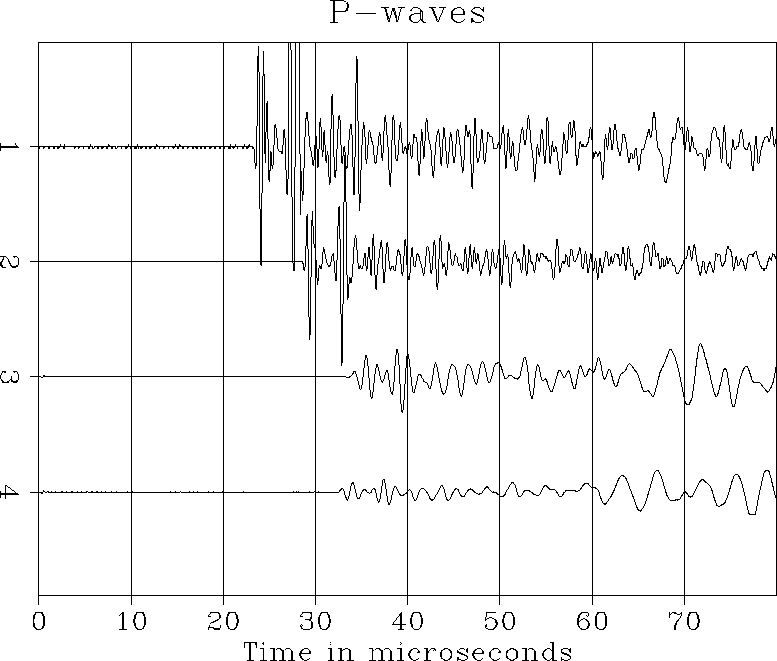
Figure shows an example of compressional waveforms measured across
different core samples in a lab experiment,
Lumley et al. .
These measurements may be repeated under varying lab conditions of
confining pressure and temperature to map out the response of a dry
rock sample to reservoir pore pressure and temperature.
Based on the dry
are computed.
Figure shows an example of compressional waveforms measured across
different core samples in a lab experiment,
Lumley et al. .
These measurements may be repeated under varying lab conditions of
confining pressure and temperature to map out the response of a dry
rock sample to reservoir pore pressure and temperature.
Based on the dry ![]() ,
, ![]() and
and ![]() data, the dry
bulk moduli Kdry and dry shear moduli Gdry of the core samples
can be obtained using the relation:
data, the dry
bulk moduli Kdry and dry shear moduli Gdry of the core samples
can be obtained using the relation:
| |
(6) |
where ![]() is the dry density.
is the dry density.
 |
Saturated rock properties
Unfortunately, ultrasonic lab measurements of saturated rock properties are not representative of field saturated rock properties in the surface-seismic frequency bandwidth (10-200 Hz). This is due to dispersive wave effects caused by frequency-dependent fluid oscillations in the core sample pore space at ultrasonic frequencies. However, the velocity effect of saturation can be calculated at seismic frequencies by using Gassmann's formulas, e.g., Bourbié et al. . This formula relates the effective elastic moduli of a dry rock to the effective moduli of the same rock containing fluid at low frequencies:
| |
(7) |
| |
(8) |
where Ksat and Gsat are the effective bulk and shear moduli
of the saturated rock.
Gassmann's relations require knowledge of the
effective shear and bulk moduli of the dry rock (Gdry and Kdry),
the bulk modulus of the mineral material making up the rock (Ksolid),
the effective bulk modulus of the saturating pore fluid (Kfluid),
and the porosity ![]() .
Equation (7) is used to compute the low-frequency
bulk modulus of saturated rock from high-frequency dry rock data.
.
Equation (7) is used to compute the low-frequency
bulk modulus of saturated rock from high-frequency dry rock data.
For partially saturated rocks at sufficiently low frequencies, we can use an effective modulus Kfluid for the pore fluid that is an isostress average of the moduli of the liquid and gaseous phases:
| |
(9) |
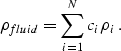
This requires knowledge of the bulk modulus of the liquid phase (Kliquid), the bulk modulus of the gas phase (Kgas), and the saturation values (S). In general, if the pore fluid includes more than two phases, we can calculate the mixture's effective bulk modulus Kfluid based on the the number of fluid components N, the volumetric concentrations ci of the ith component, and their bulk moduli Ki:
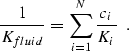 |
(10) |
Finally, we can use the following formulas to find seismic velocities in saturated rocks:
 |
(11) |
 |
(12) |
where ![]() is the density of the saturated rock:
is the density of the saturated rock:
| |
(13) |
![]() is the density of the solid phase, and
is the density of the solid phase, and
![]() is the density of the fluid mixture obtained as an
arithmetic mean of the volume-concentration-weighted fluid density
components
is the density of the fluid mixture obtained as an
arithmetic mean of the volume-concentration-weighted fluid density
components ![]() :
:
 |
(14) |
SEISMIC WAVE THEORY
Given the fluid-flow pressure, temperature and saturation data, mapped to seismic P-wave and S-wave velocity and density, the response of these fluid-flow changes can be modeled and imaged in seismic data by considering basic elastic wave theory.
Elastic wave modeling
Consider the elastodynamic wave equation for a seismic particle
displacement vector wavefield ![]() and a second order
tensor stress field
and a second order
tensor stress field ![]() due to a body force vector excitation
due to a body force vector excitation ![]() :
:
| |
(15) |
e.g., Aki and Richards . Assume further a linear elastic stress-strain relationship in the material continuum such that
| |
(16) |
where ![]() is the fourth-order elastic stiffness tensor Cijkl,
and the ``
is the fourth-order elastic stiffness tensor Cijkl,
and the ``![]() '' symbol means a second order inner contraction.
A volume integral representation for the
'' symbol means a second order inner contraction.
A volume integral representation for the ![]() ``P-wave to P-wave'' scattered
wavefield
``P-wave to P-wave'' scattered
wavefield ![]() can be expressed as:
can be expressed as:
| |
(17) |
Equation (17) is the volume integral representation of the reflected
![]() wavefield
wavefield ![]() measured at a receiver
measured at a receiver ![]() along
an arbitrary
vector component direction
along
an arbitrary
vector component direction ![]() , due to the excitation of a
body force reflection-diffraction scattering potential
, due to the excitation of a
body force reflection-diffraction scattering potential ![]() at each subsurface point
at each subsurface point ![]() ,
excited by the incident source wavefield
,
excited by the incident source wavefield ![]() generated by a
seismic source located at
generated by a
seismic source located at ![]() .
.
The assumption of isotropic elastic WKBJ (ray-valid) Green's tensors for P waves leads to:
| |
(18) |
where A<<701>>P and ![]() are the ray-valid P-wave amplitude and traveltime
from the ``source'' location
are the ray-valid P-wave amplitude and traveltime
from the ``source'' location ![]() to the ``observation'' point
to the ``observation'' point ![]() ,
and are related by the eikonal and transport equations respectively:
,
and are related by the eikonal and transport equations respectively:
| |
(19) |
| |
(20) |
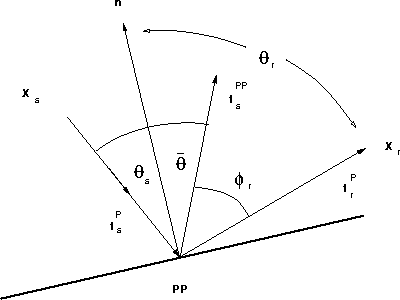
The unit vector ![]() is the direction parallel to P-wave propagation,
as shown in Figure ,
and is perpendicular to the wavefronts
is the direction parallel to P-wave propagation,
as shown in Figure ,
and is perpendicular to the wavefronts ![]() .
.
For a linear isotropic elastic solid, the stress-strain relationship is
| |
(21) |
where ![]() and
and ![]() are the Lamé parameters such that
are the Lamé parameters such that
| |
(22) |
and ![]() is the second-order identity matrix
is the second-order identity matrix ![]() .Lumley and Beydoun showed that the P-wave
reflection-diffraction scattering potential
.Lumley and Beydoun showed that the P-wave
reflection-diffraction scattering potential ![]() is:
is:
| |
(23) |
Equation (23) is a body force equivalent for
scattering-surface reflectivity
excitations, and is clearly dependent on material property contrasts
(gradients): ![]() ,
, ![]() and
and ![]() .
.
After some algebraic manipulation, (17) can be represented as:
| |
(24) |
To recap (24), the density at a
subsurface point is denoted ![]() , and the geometric reflection coefficient
at that point is
, and the geometric reflection coefficient
at that point is ![]() . The amplitude terms As and Ar represent
the cumulative geometric spreading, transmission loss, Q-attenuation, etc.,
from the source and receiver to the subsurface point
. The amplitude terms As and Ar represent
the cumulative geometric spreading, transmission loss, Q-attenuation, etc.,
from the source and receiver to the subsurface point ![]() respectively.
The factor
respectively.
The factor ![]() involves the vector component projection at the surface
location
involves the vector component projection at the surface
location ![]() of
of ![]() onto the arbitrary direction
onto the arbitrary direction ![]() .The term
.The term ![]() is the total traveltime from the source
at
is the total traveltime from the source
at ![]() to the subsurface point
to the subsurface point ![]() and back up to the receiver at
and back up to the receiver at ![]() .Finally, the diffraction weight
.Finally, the diffraction weight ![]() represents the angle between the anticipated geometric specular reflection
direction
represents the angle between the anticipated geometric specular reflection
direction ![]() and the non-geometric diffraction direction
and the non-geometric diffraction direction ![]() .
In the case
of specular reflection when
.
In the case
of specular reflection when ![]() ,
, ![]() and so
and so ![]() .The generalized reflection ray and angle geometries are shown in
Figure .
.The generalized reflection ray and angle geometries are shown in
Figure .
A linearized version of the nonlinear ![]() reflection coefficient
can be parameterized as:
reflection coefficient
can be parameterized as:
| |
(25) |
where ![]() and
and ![]() is the reflection angle between
the incident wave direction
is the reflection angle between
the incident wave direction ![]() and the local gradient of the
compressional P-impedance structure
and the local gradient of the
compressional P-impedance structure ![]() .This linearization is also given in a somewhat different parameterization by
Aki and Richards ,
and is accurate when the relative perturbations
in impedance and density are small,
and the reflection angles
.This linearization is also given in a somewhat different parameterization by
Aki and Richards ,
and is accurate when the relative perturbations
in impedance and density are small,
and the reflection angles ![]() are less than the critical angle
at which conical ``head waves'' emerge.
are less than the critical angle
at which conical ``head waves'' emerge.
The seismic modeling equations (19), (20),
(24) and (25)
show that changes in fluid-flow pressure, temperature and saturation,
mapped to ![]() ,
, ![]() and
and ![]() changes through rock physics transformations,
will have an effect on the traveltimes
changes through rock physics transformations,
will have an effect on the traveltimes ![]() and reflection amplitudes
and reflection amplitudes
![]() in the seismic data
in the seismic data ![]() . If several seismic surveys are
recorded at different phases of production fluid-flow, the seismic
response will change with calendar time due to the coupled equations
in fluid-flow, rock physics and elastic wave theory shown above.
For example,
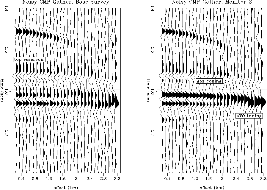
Figure shows modeled CMP gather
seismograms, after moveout correction, before and after oil production
from a horizontal well.
The next section addresses the topic of imaging changes in fluid-flow
directly from multiple seismic data sets recorded in ``monitoring'' mode.
. If several seismic surveys are
recorded at different phases of production fluid-flow, the seismic
response will change with calendar time due to the coupled equations
in fluid-flow, rock physics and elastic wave theory shown above.
For example,
Figure shows modeled CMP gather
seismograms, after moveout correction, before and after oil production
from a horizontal well.
The next section addresses the topic of imaging changes in fluid-flow
directly from multiple seismic data sets recorded in ``monitoring'' mode.
 |
 |
Seismic wavefield imaging
Given a seismic data set recorded at some calendar time T1, we would like to be able to image the subsurface reflectivity structure R1 which generated the reflected waves observed in that seismic data. Furthermore, we would like to obtain several reflectivity estimates R1, R2, R3,... corresponding to surveys over a producing reservoir at calendar times T1, T2, T3..., and infer something about the change in subsurface fluid flow from the changes in the Ri maps. The required imaging procedure is called ``seismic migration'' in the seismic exploration industry.
I briefly derive a ``kinematic'' Kirchhoff prestack depth migration equation which is suitable for either 2-D or 3-D data acquisition, and incorporates single-arrival traveltime and phase estimates. This migration equation yields accurate estimates of reflectivity amplitudes for near-offset data, and provides an efficient and robust structural imaging condition for far-offset data, Lumley .
Given the Helmholtz variable-velocity ![]() scalar wave equation
scalar wave equation
| |
(26) |
the ``downgoing wavefield'' D generated by a single source at location
![]() can be evaluated at any subsurface location
can be evaluated at any subsurface location ![]() within a volume
within a volume
![]() from the frequency-domain integral representation:
from the frequency-domain integral representation:
| |
(27) |
where ![]() is the Green's function solution to (26)
associated with the source location, and S is the source wave function.
If we neglect the
absolute amplitude of the source and consider only relative amplitudes
in the migrated section, and assume the source has a compact delta
function shape in both space and time:
is the Green's function solution to (26)
associated with the source location, and S is the source wave function.
If we neglect the
absolute amplitude of the source and consider only relative amplitudes
in the migrated section, and assume the source has a compact delta
function shape in both space and time: ![]() ,
then the downgoing wavefield
can be approximated by the source Green's function alone:
,
then the downgoing wavefield
can be approximated by the source Green's function alone:
![]() .
.
The ``upgoing wavefield'' U reflected from the subsurface ![]() due to a source at
due to a source at ![]() can be reconstructed from the seismic
(scalar) data
can be reconstructed from the seismic
(scalar) data ![]() recorded at receivers
recorded at receivers ![]() using a
Kirchhoff integral representation:
using a
Kirchhoff integral representation:
| |
(28) |
where ![]() is the receiver Green's function and
is the receiver Green's function and ![]() is
the unit vector normal to the recording surface
is
the unit vector normal to the recording surface ![]() that bounds
the image volume
that bounds
the image volume ![]() of interest. The gradient operator
of interest. The gradient operator ![]() is taken with respect to the subsurface coordinate
is taken with respect to the subsurface coordinate ![]() along the
recording surface at
along the
recording surface at ![]() .
.
Given that the reflected wavefield U can be modeled as a convolution
of the subsurface reflectivity R with the source wavefield D,
a local least-squares estimate of R can be obtained as the
weighted zero-lag correlation of the source and reflected wavefields:
![]() , where W are as yet
unspecified weights, and
, where W are as yet
unspecified weights, and ![]() is the complex conjugate of D.
If this weighted zero-lag correlation is further averaged for all such
single shot-profile migrations, the frequency-domain Kirchhoff migration
equation becomes:
is the complex conjugate of D.
If this weighted zero-lag correlation is further averaged for all such
single shot-profile migrations, the frequency-domain Kirchhoff migration
equation becomes:
| |
(29) |
It can be shown that the reflectivity image R is proportional to a
reflection-angle averaged version of the ![]() coefficient in
the modeling equation (24), and is a first order estimate
of the relative P-wave impedance contrast in the earth,
coefficient in
the modeling equation (24), and is a first order estimate
of the relative P-wave impedance contrast in the earth,
![]() , as inferred from equation (25).
, as inferred from equation (25).
Assume a parametric form for the Green's functions G such that:
| |
(30) |
where opposite signs are chosen in the exponential for the source
(outgoing) and receiver (reverse-time extrapolated) Green's functions
respectively.
The parameters Aa, ![]() and
and ![]() are the single-arrival
Green's function amplitudes, traveltimes and phase rotations from location
are the single-arrival
Green's function amplitudes, traveltimes and phase rotations from location
![]() to
to ![]() . These parameters are often estimated by conventional
high-frequency asymptotic ray methods.
. These parameters are often estimated by conventional
high-frequency asymptotic ray methods.
Given the parametric form (30), an efficient time-domain version of (29) can be obtained as:
| |
(31) |
where the ``obliquity factor'' ![]() is a function of the incident angle
at each receiver with respect to the surface normal, and is
obtained as the dot product
is a function of the incident angle
at each receiver with respect to the surface normal, and is
obtained as the dot product ![]() .The Kirchhoff space-time migration equation (31) is a weighted
diffraction stack of the preprocessed, deconvolved
(but not divergence-corrected) data
.The Kirchhoff space-time migration equation (31) is a weighted
diffraction stack of the preprocessed, deconvolved
(but not divergence-corrected) data ![]() , after phase-rotation by
the Green's function parameters
, after phase-rotation by
the Green's function parameters ![]() , evaluated
along the diffraction trajectories given by the Green's function
traveltimes
, evaluated
along the diffraction trajectories given by the Green's function
traveltimes ![]() .
.
I define kinematic migration by setting the migration weights
![]() to unity.
I note that (31) is suitable for 2-D migration if all
spatial coordinates are 2-vectors, e.g.
to unity.
I note that (31) is suitable for 2-D migration if all
spatial coordinates are 2-vectors, e.g. ![]() , and
, and
![]() is preprocessed by the half-time derivative operator
is preprocessed by the half-time derivative operator ![]() .
However, (31) is equally suitable for 3-D migration if
all spatial coordinates are 3-vectors, e.g.
.
However, (31) is equally suitable for 3-D migration if
all spatial coordinates are 3-vectors, e.g. ![]() , and
, and
![]() is preprocessed by the full time derivative
is preprocessed by the full time derivative ![]() .
.
Seismic velocity analysis
The seismic migration equation (31) images subsurface
reflectivity structure, which is proportional to short-wavelength
impedance variation. However, (31) is a nonlinear function of wave
propagation velocity ![]() to first order in traveltimes
to first order in traveltimes ![]() ,
and to second order in amplitudes A. The coherency of any reflectivity image
is therefore dependent upon the accuracy to which the long-wavelength velocity
structure
,
and to second order in amplitudes A. The coherency of any reflectivity image
is therefore dependent upon the accuracy to which the long-wavelength velocity
structure ![]() is known.
Velocity estimation is nonlinear, and reflectivity estimation
is linear, given a smooth estimate of the background velocity field.
In general, the problem of estimating the
short-wavelength reflectivity and the long-wavelength velocity are
nonlinearly coupled, and need to be solved simultaneously.
In practice, the problem is usually assumed to be separable and solved
separately; first for the velocity and then for the reflectivity.
is known.
Velocity estimation is nonlinear, and reflectivity estimation
is linear, given a smooth estimate of the background velocity field.
In general, the problem of estimating the
short-wavelength reflectivity and the long-wavelength velocity are
nonlinearly coupled, and need to be solved simultaneously.
In practice, the problem is usually assumed to be separable and solved
separately; first for the velocity and then for the reflectivity.
A general nonlinear inverse problem can be posed to solve for
long-wavelength velocity and short-wavelength impedance as follows.
A measure of coherency can be defined as some function ![]() of the
reflectivity image R, which is itself a function of the velocity
of the
reflectivity image R, which is itself a function of the velocity ![]() ,
,
| |
(32) |
Since the image is assumed to be most coherent at the correct velocity model, a nonlinear optimization problem ensues, e.g., Symes and Carazzone . An optimal velocity solution is obtained when the coherency does not improve with slight adjustments to the velocity model:
| |
(33) |
Equation (33) is the gradient of the image coherency with respect to velocity perturbation, and can be used in a nonlinear steepest-descent or conjugate-gradient method to iterate towards a final solution.
Seismic fluid-flow monitoring
The seismic migration equation (31) can be used to obtain an estimate
of the subsurface reflectivity R for any seismic data set.
This reflectivity image is an angle-average estimate of the elastic
![]() scattering coefficient, and is a first order estimate of
short-wavelength P-wave impedance contrasts,
scattering coefficient, and is a first order estimate of
short-wavelength P-wave impedance contrasts, ![]() , in
the subsurface. Information on the long-wavelength velocity structure
, in
the subsurface. Information on the long-wavelength velocity structure
![]() is available in the seismic data from the traveltime information
is available in the seismic data from the traveltime information
![]() in the wavefield
in the wavefield ![]() , by solution of the nonlinear
velocity analysis system (33).
The velocity structure
, by solution of the nonlinear
velocity analysis system (33).
The velocity structure ![]() and reflectivity image R estimated
from a single seismic survey will be comprised of coupled contributions
from the reservoir geology and the fluid-flow states in pore space.
The estimation and interpretation
of this information from a single seismic data set is known as seismic
reservoir characterization:
and reflectivity image R estimated
from a single seismic survey will be comprised of coupled contributions
from the reservoir geology and the fluid-flow states in pore space.
The estimation and interpretation
of this information from a single seismic data set is known as seismic
reservoir characterization:
![]()
Seismic reservoir characterization is a very difficult task because of the ambiguity in trying to separate geology effects from fluid-flow effects in a single seismic data set.
However, when multiple seismic surveys are conducted at separate
calendar times, it is expected that the reservoir geology will
not change from survey to survey, but the state of fluid flow will change.
Therefore, differencing a series of reflectivity images Ri and velocity model
estimates ![]() will remove the static geologic contribution to the seismic
data, and isolate time-varying seismic changes in the reservoir which
are due to time-varying fluid-flow changes alone. The process of
estimating and comparing reflectivity images and velocity estimates
from multiple seismic data sets recorded at different calendar times
is known as seismic reservoir monitoring,
will remove the static geologic contribution to the seismic
data, and isolate time-varying seismic changes in the reservoir which
are due to time-varying fluid-flow changes alone. The process of
estimating and comparing reflectivity images and velocity estimates
from multiple seismic data sets recorded at different calendar times
is known as seismic reservoir monitoring,
![]()
Seismic reservoir monitoring is potentially a much less ambiguous task than characterization, because the effects of geology and fluid-flow may be uncoupled by comparing time-varying seismic data sets.
SYNTHETIC EXAMPLE
In this section, I present a simulated example of seismic reservoir monitoring on a North Sea reservoir, Lumley et al. , in order to determine if it would be feasible to observe changes in seismic monitor data given a specific fluid flow and reservoir geology scenario. Fluid-flow simulations were computed by Norsk Hydro for the case of solution-gas-drive oil production from a horizontal well in the reservoir after 56 and 113 days of production. Reservoir geology and core data measurements were combined to make rock physics transformations of the fluid-flow saturation, pressure and temperature data to seismic velocities and densities. Multi-offset elastic reflection seismogram surveys were simulated at each production phase. Prestack migration images show gas coning during production in reasonable seismic noise levels and frequency bandwidth.
Fluid-flow simulation
The oil zone is located at a depth of approximately 1550 meters,
and it varies in thickness from a few meters to more than 20 meters.
Horizontal drilling technology makes it possible to commercially produce oil
from this thin oil zone.
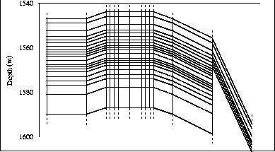
The reservoir fluid-flow grid, shown in Figure ,
consisted of 312 individual blocks, and each grid cell was given with a
fluid-flow simulation data value of porosity, pore pressure, gas saturation,
oil saturation, and water saturation. As an example of the simulation data,
Figure shows the change in oil saturation after
113 days of production.
The thin oil zone is compressed due to gascap expansion from above
and upward water coning from below.
 |
Rock physics
Given the fluid-flow simulation data and reservoir geology,
rock physics analysis is used to transform pressure, temperature and saturation
data into ![]() ,
, ![]() and
and ![]() distributions within the reservoir.
Estimates of dry rock properties in the reservoir are based on the
results in a similar reservoir reported by Blangy and Strandenes
and Blangy ,
which involved laboratory experiments conducted on 38 core samples.
Figure shows an example
of the
distributions within the reservoir.
Estimates of dry rock properties in the reservoir are based on the
results in a similar reservoir reported by Blangy and Strandenes
and Blangy ,
which involved laboratory experiments conducted on 38 core samples.
Figure shows an example
of the ![]() core measurements made as a function of reservoir
sand porosity at 20 MPa differential pressure.
core measurements made as a function of reservoir
sand porosity at 20 MPa differential pressure.
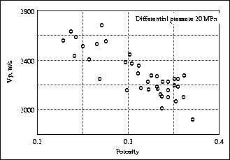 |
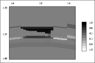
Figure shows an example of the change in P impedance
mapped from the fluid-flow simulation at 113 days of oil production
compared to the the initial reservoir state prior to production.
There is a significant decrease in P impedance above the oil zone where the
gascap has expanded downward, and a smaller increase in P impedance below the
oil zone where the aquifer has coned upward during production.
The maximum relative decrease in P impedance is about 15% which is
strong enough to cause a significant seismic reflection.
 |
Seismic monitoring
Given the ![]() ,
, ![]() and
and ![]() distributions in the reservoir
corresponding to the fluid-flow simulation data and rock physics
transformations, I simulated a multi-offset surface seismic survey at each
of three separate monitoring phases of oil production.
These three prestack datasets were then
processed to produce stacked and prestack-migrated
reflectivity images. Difference images obtained by subtracting combinations
of stacked and migrated sections clearly show that reservoir fluid production
is visible in the seismic data and can be monitored in the presence of
reasonable levels of seismic noise.
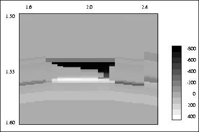
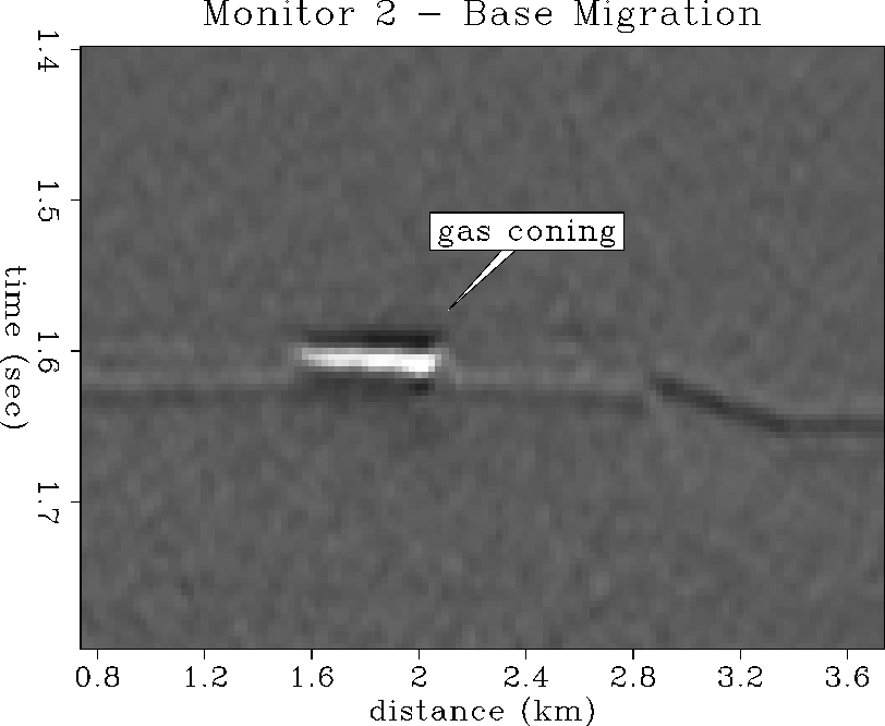
Figure shows the difference section obtained by
a simple subtraction of
the Base Survey migration image, prior to oil production, from the Monitor 2
migration image, after 113 days of oil production.
The gas coning clearly stands out from the background seismic noise as a
bright spot at 2 km and 1.6 s, and accurately defines the spatial
extent of the true impedance model anomaly.
distributions in the reservoir
corresponding to the fluid-flow simulation data and rock physics
transformations, I simulated a multi-offset surface seismic survey at each
of three separate monitoring phases of oil production.
These three prestack datasets were then
processed to produce stacked and prestack-migrated
reflectivity images. Difference images obtained by subtracting combinations
of stacked and migrated sections clearly show that reservoir fluid production
is visible in the seismic data and can be monitored in the presence of
reasonable levels of seismic noise.
Figure shows the difference section obtained by
a simple subtraction of
the Base Survey migration image, prior to oil production, from the Monitor 2
migration image, after 113 days of oil production.
The gas coning clearly stands out from the background seismic noise as a
bright spot at 2 km and 1.6 s, and accurately defines the spatial
extent of the true impedance model anomaly.
 |
FIELD DATA EXAMPLE
In this section I briefly show a field data example from a steamflood in the Duri field, Indonesia, first reported by Bee et al. and Lumley .
Field data
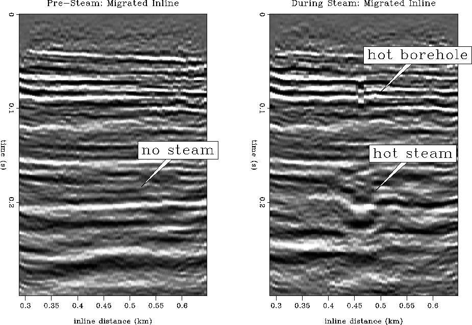
Figure shows two inline profile-view sections
cut from a 3-D migration cube. The left panel is before
steam injection, the right panel is after 5 months of steam injection.
After steam injection, the heat, pressure and desaturation of the
steamed zone show up clearly as differences in the time-lapse
seismic sections. The shallow portion of the borehole is even
visible in the seismic data due to heating of the casing and surrounding rock.
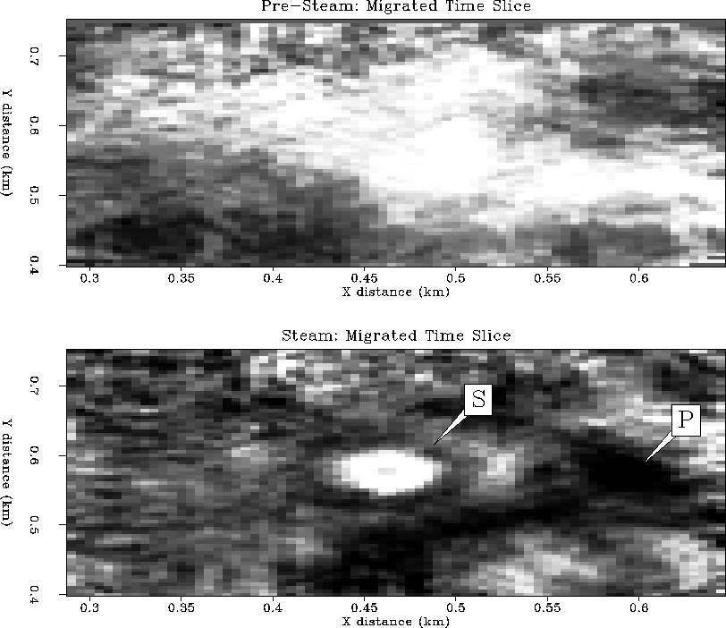
Figure shows two time-slice map-view sections
cut from a 3-D migration cube at about the depth that steam should be
penetrating the reservoir. The lower panel shows a circular disk
of steam ``S'' about 50 m in diameter (white), and a large outer annulus
interpreted to be a transient pressure front ``P'' (dark gray).
These examples clearly demonstrate that reservoir fluid-flow changes
can be seen in some field conditions with time-lapse seismic
monitor data.
CONCLUSION
I have discussed the physical theory relevant for three-phase fluid flow in a producing oil reservoir, and rock physics transformations of fluid-flow pressure, temperature and pore-fluid saturation values to seismic P-wave and S-wave velocity. I have linked fluid-flow physical parameters to seismic reflection data amplitudes and traveltimes through elastic wave equation modeling and imaging theory. I have demonstrated with both synthetic and field data examples that changes in fluid-flow can be monitored and imaged in certain conditions from repeated seismic surveys acquired at varying production calendar times.
ACKNOWLEDGMENTS
I thank Amos Nur, Jack Dvorkin and James Packwood of the Stanford Rock Physics Laboratory for their collaboration on the synthetic data example. Sverre Strandenes and Norsk Hydro were very helpful in providing the reservoir geology information and fluid-flow simulation data. The steamflood data were kindly provided by Steve Jenkins (CalTex), and Fred Herkenhoff and Ray Ergas (Chevron).
 |
 |
[MISC,GEOTLE,GEOPHYSICS,SEGCON,SEP]