 |
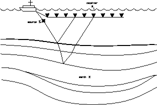
Figure 1 Ship pulling a streamer during a marine survey.
![[*]](http://sepwww.stanford.edu/latex2html/prev_gr.gif)
ABSTRACTSource and receiver amplitude variations can distort AVO analysis of prestack seismic reflection data. We therefore perform an amplitude balancing of seismic traces from a marine data set. We address this problem by computing the total energy of each trace in the seismic survey, and remove the global low-wavenumber amplitude trend from the resulting 2-D trace energy map. We then estimate an amplitude coefficient for each physical hydrophone position in the recording cable, and each shot position along the survey line. We apply these coefficients to the original seismic traces and successfully remove most of the source and receiver amplitude variation. |
INTRODUCTION
Ultimately, we plan to perform an AVO analysis on the data set provided by Mobil. However, some care needs to be taken in the preprocessing stages to ensure that amplitude information is correct. In particular, we address the issue of source and receiver amplitude balancing.
The marine cable used to record the Mobil data consisted of hydrophones of varying amplitude response. Some receivers are relatively weaker or stronger than others. Additionally, some of the source strengths vary along the survey line, due to varying air gun pressure and misfires. Therefore, amplitude balancing of the traces is necessary. Yu has discussed an amplitude balancing method. We assume a simple amplitude model where receiver amplitudes are constant for all shot locations at a given hydrophone position in the cable. Similarly, we assume that a source amplitude is constant for all receivers at a particular shot location.
To perform a non-biased AVO analysis, we need to estimate these source and receiver amplitude responses, and compensate the prestack traces accordingly. We first calculate the total integrated energy for each trace in the survey. Then we remove the global low-wavenumber trend of this 2-D trace energy map. Finally, we determine the source and receiver amplitude balancing coefficients for each shot and receiver, and apply them to balance the original prestack data.
AN AMPLITUDE BALANCING MODEL
In the field, acquisition systems used in seismic exploration surveys are composed essentially of a source S that generates waves and receivers Ri which are geophones on land or hydrophones in the sea.
In a marine survey, the receivers are lined up in a streamer pulled by the ship. Figure survey shows a ship performing a marine seismic survey.
 |
For a shot gather, each trace recorded at the receiver Ri can be interpreted as the result of the convolution of the source impulse wavelet S with the earth model E and with the receiver impulse response Ri:
| (1) |
Receiver impulse responses vary along the cable, some of them are stronger, others are weaker.
We want to test different AVO schemes on the Mobil data set. Because the traces recorded by some receivers have an amplitude which seems to be too different from the average response of the other receivers, it is necessary to correct for these anomalies before doing the AVO analysis, and increase or decrease the amplitude of the corresponding receivers in each shot gather. This operation is called ``balancing the cable'' since we want to obtain amplitudes that would have been recorded by a cable made of ideal copies of a unique receiver.
In the following two sections, we consider that the total trace energy obtained by summing the squared amplitudes along the time axis satisfy the following model:
| |
(2) |
Taking the logarithm of expression (2), we have:
| (3) |
After correcting atotal for the low-wavenumber trend of Aearth, we should obtain:
| |
(4) |
REMOVING THE GLOBAL AMPLITUDE TREND
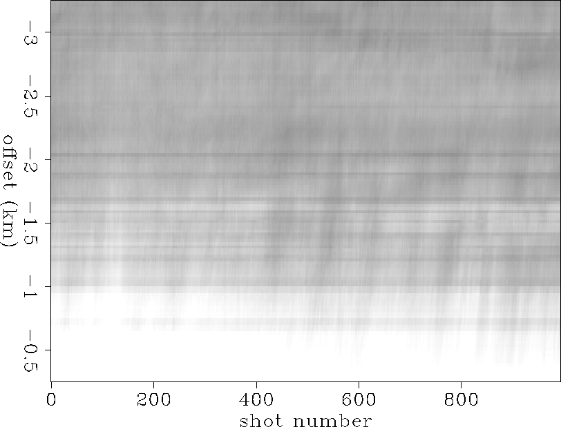
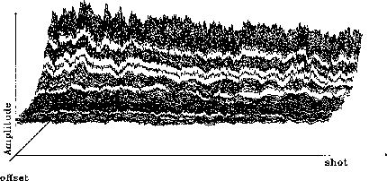
We first calculate the total integrated energy for each trace of the survey by summing the amplitudes of the traces over the time axis. Figure amplitude shows an amplitude plot as a function of offset and shot number. This amplitude plot has been obtained by taking the square root of the 2-D energy map. In Figure amp3d the same amplitude function is represented as a 2-D surface. Its shape has a global exponential decay in the offset direction and a linear trend in the shot direction.
 |
 |
The plot of the 2-D amplitude function (Figure amplitude) shows horizontal stripes parallel to the shot direction, visible especially around an offset of -1.5 km, and some less visible vertical stripes parallel to the offset direction. These horizontal and vertical lines correspond respectively to variations of the impulse response of some receivers and variations of source strength. In order to estimate the receiver and shot response, we first remove the global trend in the 2-D amplitude function.
Removing the trend in the offset direction
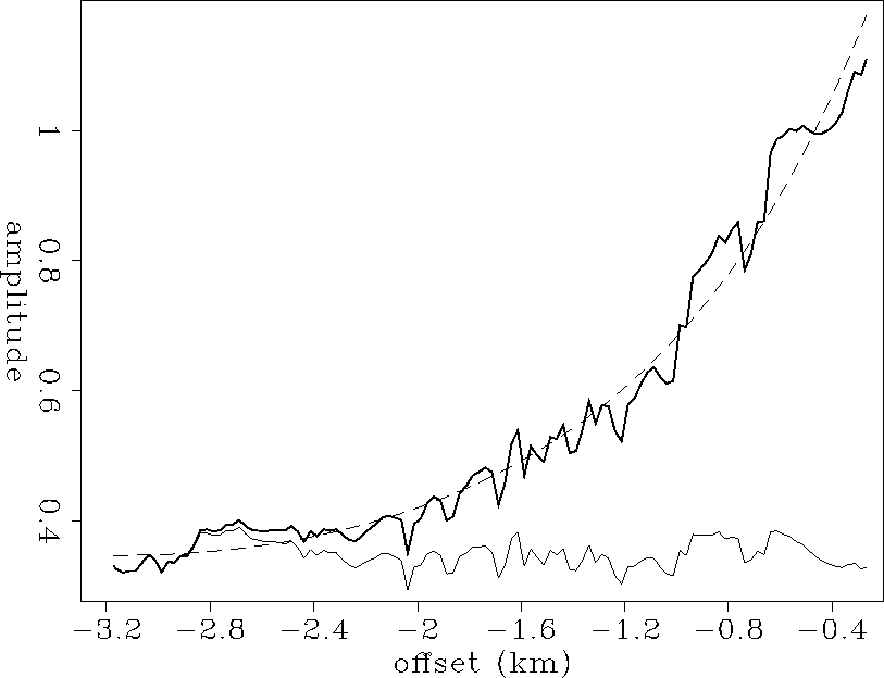
In the offset direction, the amplitude curve for a representative shot is plotted as the thick solid line in Figure shot120. We want to remove the global trend of this curve to reveal the residuals.
As a first approach we tried to obtain a smooth version of the 1-D amplitude curve by applying the SEP Smooth program with a four-point triangle filter, and low-pass filtering in the wavelet domain. These methods did not produce results accurate enough so far, but may be the subject of further investigation.
The general shape of these curves leads us to fit an exponential function of offset:
| (5) |
 |
In order to flatten out the original amplitude curve, we multiply it by a correction coefficient:
| |
(6) |
Figure shot120 shows the result we obtain for the amplitude curve corresponding to shot number 120. The values of the estimated coefficients for the least-squares fitting curve are:
 |
(7) |
The same method has been applied to the entire 2-D amplitude plane. A best-fitting curve has been estimated in the offset direction for each shot point, and removed from the original amplitude in order to flatten out the amplitude surface in the offset direction.
Removing the trend in the shot direction
In Figure offset120, the thick curve is the amplitude for the nearest offset (offset -0.2375 km) as a function of shot coordinate. The global shape of the amplitude curves in the shot direction is less complicated than in the offset direction (see Figure amp3d). We approximated it by the linear function:
| (8) |
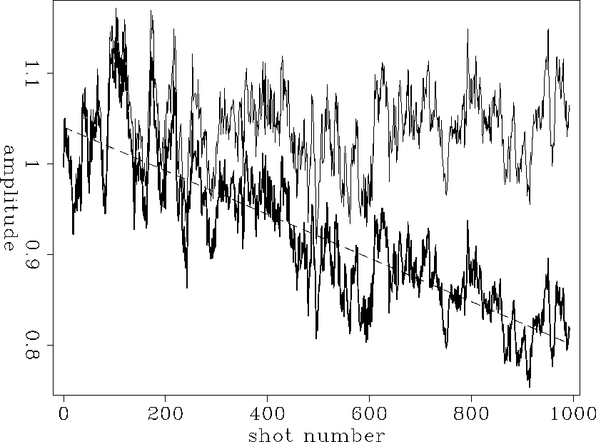 |
The estimated value of the coefficients are for the amplitude curve corresponding to the nearest offset the following:
| (9) |
This technique is then applied to the 2-D amplitude plane. A best-fitting curve has been estimated in the shot direction for each offset, and removed from the original amplitude in order to flatten out the amplitude surface in the shot direction.
Comments on the result
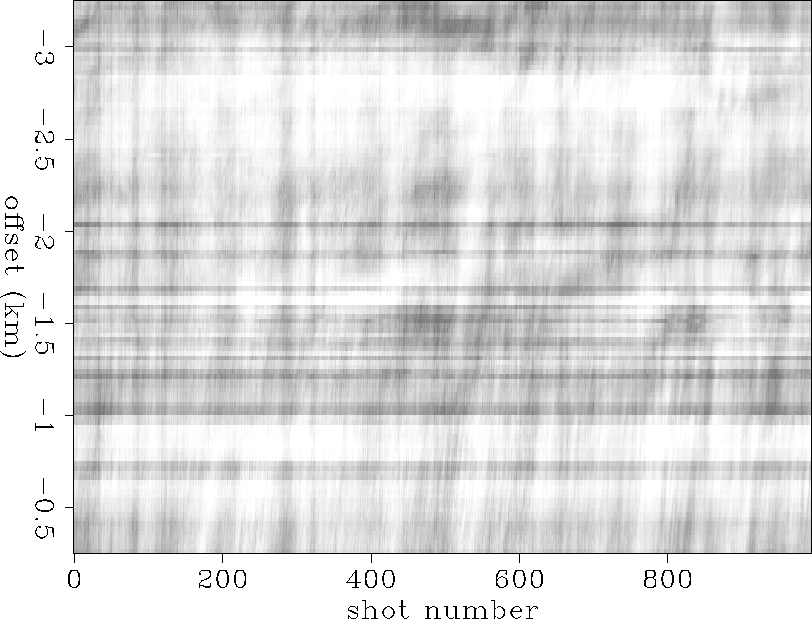 |
Figure trend shows the amplitude plane after the removal of its global trend. Removing the exponential trend in the offset direction and the linear trend in the shot direction leaves a globally flat 2-D amplitude surface with some high-frequency amplitude variation. The flattened amplitude surface presents a uniform grey background, and stripes in the receiver and shot directions have become more apparent. The grey background can be interpreted as an average response of the shots and receivers, and the component of the amplitude due to the geology as described in equation (2). The horizontal stripes correspond to receivers with an amplitude response that deviates from the global average. The vertical stripes correspond to variations of the source energy. Both of these variations have to be corrected for a subsequent AVO analysis.
AMPLITUDE BALANCING
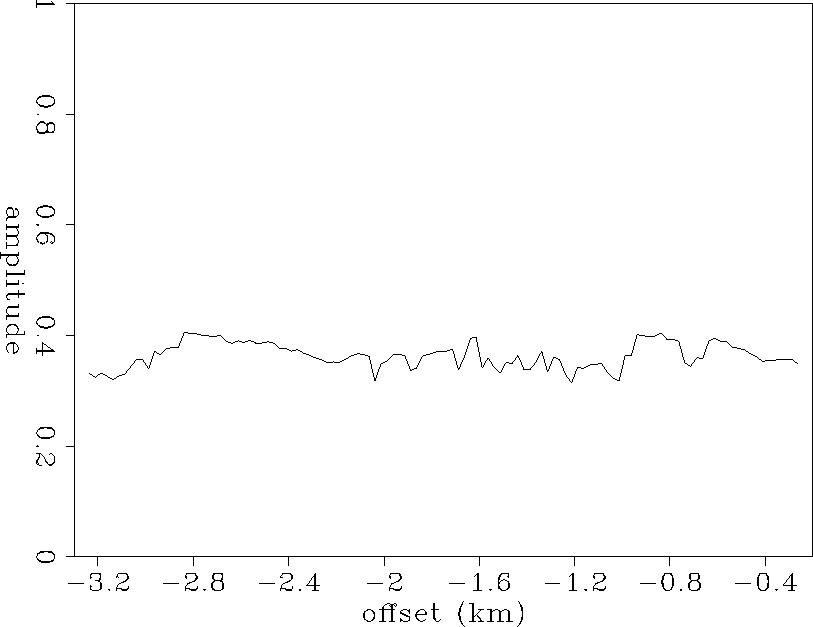
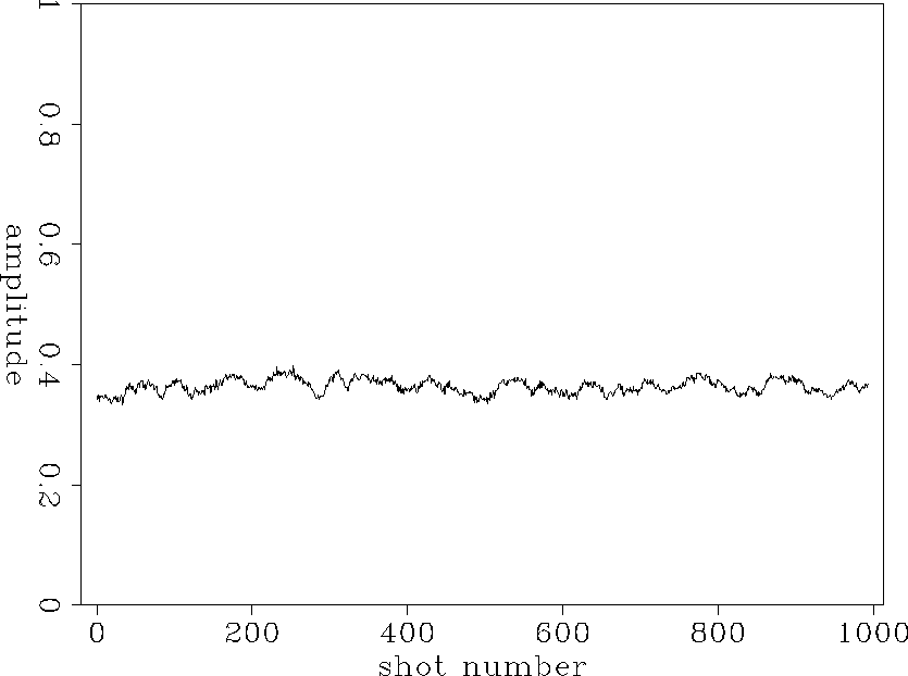
Starting with the amplitude plane shown in Figure trend, we estimate the correction coefficients in both directions that have to be applied to the data in order to remove the variations. We stack the corrected amplitude surface in the shot direction to obtain the receiver coefficients (Figure offset-coef) and in the offset direction to obtain the shot coefficients (Figure shot-coef).
 |
 |
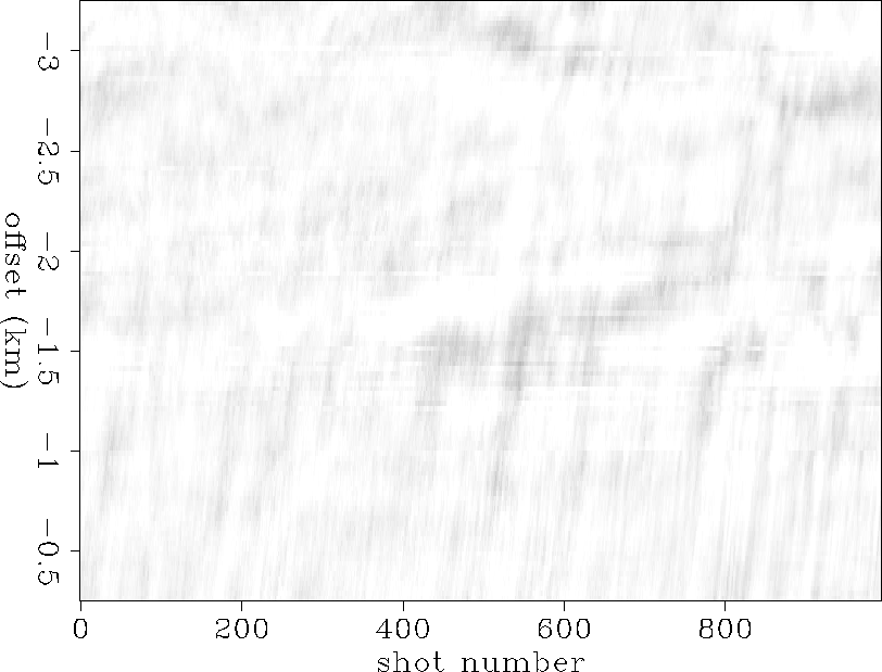
We then use these coefficients to remove the stripes from the plot in Figure trend. Figure rem shows the amplitude plot obtained after dividing the 2-D flattened amplitude of Figure trend by the coefficients in the offset and shot directions. This shows the contribution of the earth components to the amplitude of the traces recorded during the survey. Aside from this earth contribution, some residual noise, and receiver and source variations might still be present but not dominant.
 |
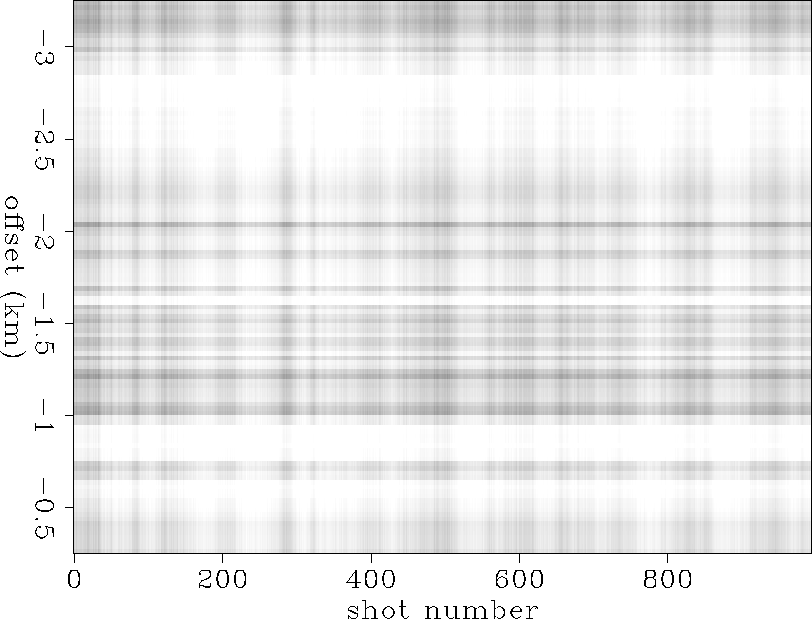 |
Figure stripes represents only the stripes, corresponding to the plane of the combined shot and receiver amplitude coefficients, Ar(h) As(s).
CONCLUSIONS
We have assumed a simple amplitude model in which receiver amplitudes are constant at a given hydrophone position in the cable for all shot locations, and source amplitudes are constant for all receivers at a particular shot location. The method of amplitude balancing resulting from this assumption produces good results. We removed the strong variations of the receiver and source components as shown on the amplitude plots (Figure rem). Our amplitude balancing can be useful in order to perform a good AVO analysis. We plan to investigate other methods of amplitude balancing, including wavelet transforms.
[GEOTLE]
![[*]](http://sepwww.stanford.edu/latex2html/prev_gr.gif)