LEAST-SQUARES SLANT STACK TRANSFORMS

The conventional slant-stack transform takes us from the recorded data d(x,t) to the slant stack domain $m(p,\tau)$:

L d = m.

In the frequency domain, a separate system of equations can be constructed for each frequency. The matrix L contains time shifts, expressed as complex exponentials:

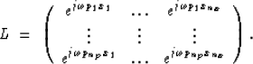$$L \ = \ \left ( \begin{array} {ccc} e^{j \omega p_1 x_1 } & ... ...\ldots & e^{j \omega p_{n_p} x_{n_x} } \\ \end{array}\right ) .$$ (2)

The conjugate operator L^H brings us back to time and space:

L^H m = d.

The conjugate operator is the more straightforward of the two. If we have a point in $(p,\tau)$ space, the operator L^H does a good job of turning it into a line in (x,t) space, regardless of the number of traces in x; there is no aperture effect. The forward transform, however, is affected by the aperture. If we transform a single dipping event in (x,t) to $(p,\tau)$ there will be artifacts and a loss of resolution, caused by the limited aperture.

We would do better to transform from (x,t) to $(p,\tau)$using the inverse of the matrix L^H:

m = (L^H)^-1 d.

However, the matrix L^H is typically not square; the problem is either overdetermined or underdetermined. In this case, we can find the best least-squares solution by multiplying both sides of the conjugate transform by L:

 

L L^H m = L d, (5)

giving:

m = ( L L^H )^-1 L d.

The matrix ( L L^H )^-1 L is the least-squares inverse of L^H.

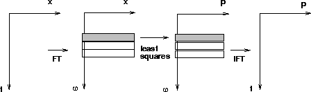
The least-squares slant stack is summarized in Figure .

 

slant
Figure 1 Schematic of least-squares slant stack. A small least-squares problem is solved for each frequency. This is less costly than working in the time domain, where one very large system of equations would need to be solved. The time-invariant moveout correction of slant stacks makes this separation possible.