SYNTHETIC EXAMPLE

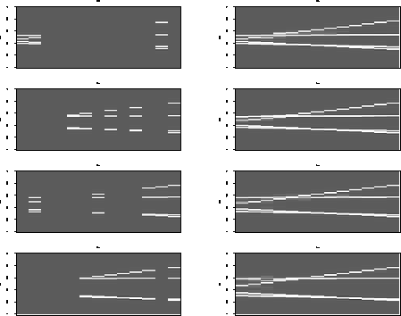
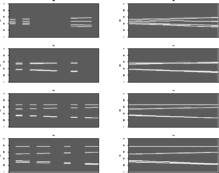
In this section, we test the algorithm on a simple synthetic dataset to illustrate its operation. Figures  and show a number of slices taken through a synthetic 3-D cube, before and after interpolation. The cube contains 13x13 traces and 128 time samples. The geometry mimics the SEP passive experiment (Nichols et al., 1989) with a 38.1 meter spacing between traces in both directions.

The dataset contains four dipping events. One is near-vertically incident (apparent velocity 8 kilometers/second). A second has a low apparent velocity of 2 km/sec, and the third and fourth are close in both apparent velocity and azimuth angle - one has an apparent velocity of 3 km/sec and a down dip azimuth of 30 degrees (relative to the x axis) while the other has an apparent velocity of 4 km/sec at an azimuth of 60 degrees. Roughly half of the 169 traces were randomly removed prior to the interpolation, which was used to restore the missing data.

In this example, and in the real data example to follow, the five nearest traces were used to construct each interpolated trace. Since the contributing traces are weighted in inverse proportion to their distance from the output location, if the output location is the same as the location of one of the contributors, that trace gets a weight of one while all others get zero weight. In other words, the interpolated result honors the input data.

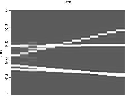
The interpolation has done a good job for the most part. Problems can be seen in a few places, such as in the crossline slice displayed at a larger scale in Figure . There the top two events, the 8 km/sec and 2 km/sec events, cross. At the crossing point there is no problem, as whichever dip is picked works fairly well for both events. But there is a problem when the two events are near one another. Then they are close enough for both dips to occur in the same small computation window used by the program. But since only one dip is picked, the treatment of the second event can be poor.

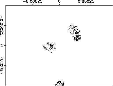
The dips picked by the algorithm are tabulated and output by the program as an optional diagnostic. A contour plot of the dips picked for the synthetic is shown in Figure . The 8 km/sec and 2 km/sec events can be seen at the center and bottom of the plot, respectively. The two events with quite similar dips give two maxima close together, in the upper right quadrant.

 

synth-xlines
Figure 3 Four crossline slices from synthetic dataset, before (left) and after interpolation.

 

synth-inlines
Figure 4 Four inline slices from synthetic dataset, before (left) and after interpolation.

 

synth-1xline
Figure 5 A single crossline slice shown at a larger scale. The only significant error occurs just to the left of the point where the top two events cross. There the two dips occur in the same computation window, but only one is picked, and the treatment of the second one (the flatter event) is poor.

 

synth-picks Figure 6 Contour plot of dips picked by algorithm as a function of px and py. The 2 km/sec and 8 km/sec events are shown at the bottom and near the center. Although not well separated in apparent velocity or azimuth, the other two events are clearly distinguishable.