IMPLEMENTATION

The steps in Claerbout's 2-D method can be summarized as follows:

• Identify a gap of missing or dead traces.
• Estimate coherence between the two traces at the ends of the gap, for all possible dips, using small overlapping time windows.
• For each time window, pick the best dip.
• Fill in each dead trace with a sum of the two end traces, each time shifted according to the dip, and weighted by distance.

In 3-D there are some additional complications. The location at which we wish to construct a trace by interpolation may not lie on a line connecting two live traces, particularly if the spatial sampling is irregular. When there is such a line, we could follow the 2-D logic and apply the prediction scheme to the two traces. This would give an estimate of the dip along that profile -- the apparent dip, not the true 3-D dip. The true dip and apparent dip are related by (Slotnick, 1959):

$$\sin \phi' = \cos (\theta - \theta') \sin \phi,$$ (1)

where $\phi$ is the true dip, $\phi'$ is the apparent dip, and $\theta$ and $\theta'$ are the azimuth angles of the down-dip direction and the direction along which the apparent dip is measured, respectively.

We could shift the two traces using this apparent dip and sum. A better idea, however, and a necessity for the case of irregular spatial sampling, is to estimate instead the true dip, using a number of nearby traces. We need at least three; from two we can only find the apparent dip in one direction.

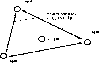
We take the three or more nearest traces, two at a time, and apply the spatial prediction operator, as in the 2-D case. This gives us the coherence as a function of the apparent dip along the direction joining the two traces. Having done these computations for each trace pair, we then loop over all possible 3-D dips (a two-dimensional space, p_x vs. p_y). For each dip, given the orientation of each trace pair, we compute what apparent dip we would see given a particular true dip. The coherence for this apparent dip is extracted from the table constructed earlier, and the coherencies are summed for all trace pairs. The result is a 2-D image of what we will call ``generalized coherence'' as a function of p_x and p_y. From this, we pick the best dip.

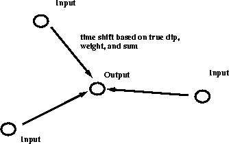
Then, for each of the neighboring traces, given the true dip, we compute the apparent dip along the line joining the trace and the location of the trace to be interpolated. This gives for each trace a time shift. The three or more neighboring traces are time shifted, weighted based on their relative distances, and summed to produce the interpolated trace.

The steps in the 3-D scheme can be summarized as follows:

• For a given output point, find the N nearest live traces.
• Estimate coherence between each pair of traces in the group, for all possible apparent dips, using small overlapping time windows. Tabulate the results.
• Loop over all 3-D dips (true dips), parameterized by p_x and p_y. For each (p_x,p_y) pair:
  • Given the true dip, compute the apparent dip between each pair of traces.
  • Extract the coherence for that apparent dip from the tables computed earlier.
  • Add coherencies for all trace pairs to get a generalized coherence for this dip.
• Scan over all (p_x,p_y) a second time to see which dip has the best coherence. Pick the best dip.
• Construct the output trace as a sum of the N neighbors, each time shifted according to the true dip, and weighted by distance.

These steps are illustrated graphically in Figures  and .

 

idraw-step1 Figure 1 Given the N nearest neighbors (here three), we first compute coherence as a function of the apparent dip between each trace pair.

 

idraw-step2 Figure 2 After deciding on the best true dip, we compute the apparent dips between each neighbor and the output, then time shift, weight, and sum.