![[*]](http://sepwww.stanford.edu/latex2html/cross_ref_motif.gif) for a geometry where sources were located
within a range of
for a geometry where sources were located
within a range of
In this section, I will show the application of the algorithm
previously explained to the inversion of
synthetic traveltimes from a cross-well geometry.
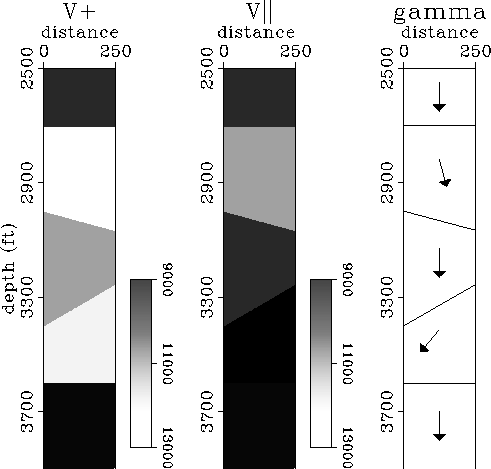
4992 traveltimes were generated through the model shown in
Figure ![[*]](http://sepwww.stanford.edu/latex2html/cross_ref_motif.gif) for a geometry where sources were located
within a range of
for a geometry where sources were located
within a range of ![]() degrees with respect to the horizontal
at each receiver position.
The ray tracing algorithm described in Michelena (1992) was
used to compute the synthetic traveltimes and to trace
the rays needed in the nonlinear inversion.
degrees with respect to the horizontal
at each receiver position.
The ray tracing algorithm described in Michelena (1992) was
used to compute the synthetic traveltimes and to trace
the rays needed in the nonlinear inversion.
 |
The starting model used for the inversion was homogeneous isotropic
described by 17 horizontal layers of equal thickness. The inclination used
for the axis of symmetry was ![]() in all layers.
Figure
in all layers.
Figure ![[*]](http://sepwww.stanford.edu/latex2html/cross_ref_motif.gif) shows the initial positions of the boundaries in the starting model.
By starting the iterations with this model I wanted
to test how the interfaces arrange themselves
to create a dipping layer not present in the initial model.
shows the initial positions of the boundaries in the starting model.
By starting the iterations with this model I wanted
to test how the interfaces arrange themselves
to create a dipping layer not present in the initial model.
 |
The inversion was constrained by not allowing parallel layers
(within ![]() degrees) to be thinner
than 15 ft. When this condition was met, the corresponding layer
was eliminated, reducing
the number of model parameters. No smoothing
was applied to the model after each iteration.
degrees) to be thinner
than 15 ft. When this condition was met, the corresponding layer
was eliminated, reducing
the number of model parameters. No smoothing
was applied to the model after each iteration.
Figure ![[*]](http://sepwww.stanford.edu/latex2html/cross_ref_motif.gif) shows the result of the inversion after
tracing rays 35 times, with few conjugate gradient iterations
between each ray tracing.
Notice how boundaries have changed positions with respect to their
initial values. Notice also that the
initial 17 layers were reduced to 10 to allow
the positioning of the dipping ones at the correct depths with the
correct dips.
The inclination of the axes of symmetry estimated
by the algorithm is also correct.
Figure
shows the result of the inversion after
tracing rays 35 times, with few conjugate gradient iterations
between each ray tracing.
Notice how boundaries have changed positions with respect to their
initial values. Notice also that the
initial 17 layers were reduced to 10 to allow
the positioning of the dipping ones at the correct depths with the
correct dips.
The inclination of the axes of symmetry estimated
by the algorithm is also correct.
Figure ![[*]](http://sepwww.stanford.edu/latex2html/cross_ref_motif.gif) compares a profile at x=0 of the
real model (Figure
compares a profile at x=0 of the
real model (Figure ![[*]](http://sepwww.stanford.edu/latex2html/cross_ref_motif.gif) ) and the estimated one
(Figure
) and the estimated one
(Figure ![[*]](http://sepwww.stanford.edu/latex2html/cross_ref_motif.gif) ). The agreement is almost perfect.
). The agreement is almost perfect.
 |
In this example, it was possible to estimate correctly both small and moderate dips (between 0 and 30 degrees), but the question of the maximum and minimum dips that can be retrieved from the data will depend in general upon the aperture of the recording geometry, the interval between sources and receivers and the frequency.