 |
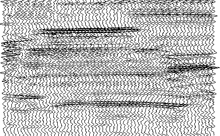
Figure 5 A wiggle trace plot.
A wide variety of displays may be generated from within Mathematica. Several auxiliary programs are available to convert displays for common terminal types. These displays may also be output to a disk file in PostScript form for use in paper documents such as this one. The YPrint.m routine in the Appendix gives one method of doing this.
While several display options are available within Mathematica,
displays may be custom-made by writing external packages from the
display primitives provided. My package to display wiggle
traces follows.
BeginPackage["Wiggle`"]

   Wiggle::usage = " plot a 2-D seismic section as a wiggle plot."
   Sigma::usage = " Get the sum of a vector."
   RMS::usage = " Get the Root mean squared of a vector."
   MRMS::usage = " Get the Root mean squared of a matrix"
   MDot::usage = " Get the dot product of a matrix with a matrix "

  Begin["`Private`"]
  Wiggle::badarg = " Bad input"

  Wiggle[a_List,s_] :=
   (
   Block[ {n,m,i,j,dim},
          dim = Dimensions[a];
          n = dim[[1]];
          m = dim[[2]];
          Show[
             Graphics[
              {
               Thickness[0.001],
               Table[Line[Table[{
                           Max[{ Min[{a[[j,i]],2 s}],-2 s}]
                                          +s j,m-i},{i,1,m}]],{j,1,n}]
              }
                     ]
              ] (* end of Show *)
         ] (* end of Block *)
   )

   Sigma[x_List] := ( Block[ {iii},
                       N[
                         Sum[ x[[iii]],{iii,1,Dimensions[x][[1]]}
                            ]
                        ]
                            ]
                    )
   RMS[x_List] := (
                       N[
                          Sqrt[ Sigma[x^2]
                            /Dimensions[x][[1]]
                              ]
                        ]
                  )

   MRMS[x_List] := (
                        N[ Sqrt[
                                Sigma[ Map[Sigma,N[x^2]] ]/
                                (Dimensions[x][[1]] Dimensions[x][[2]])
                               ]
                         ]
                   )
  MDot[x_List,y_List] := (
                       N[ Sum[
                              x[[i,j]] y[[i,j]],
                               { i,1,Dimensions[x][[1]] },
                               { j,1,Dimensions[x][[2]] }
                             ]
                        ]
                   )

End[]
EndPackage[]
Note that only the first part of this package is concerned with the actual plotting. The Sigma, RMS, MRMS, and MDot routines are used for data scaling.
To invoke Wiggle to display a matrix a, the routine is typed as follows:
Wiggle[a,MRMS[a]]
The Wiggle command takes the matrix to be plotted as the first parameter and requires a scale factor to be supplied as the second parameter. Here the routine to get the RMS of an entire matrix is used to supply the scale factor. An alternative to using MRMS[a] would be to use the maximum of the absolute values of all the values in a matrix.
Wiggle[a,Max[Abs[a]]]
If several displays are made for comparison, a numerical scale factor may be used.
Wiggle[a,3438.8]
A disadvantage of this plot is that it is slow and produces a useful result only when relatively few traces are plotted. Another disadvantage is that the axis-scales are not automatically provided. These scales might be added to the Wiggle package later. Another useful option would be a variable area addition to the wiggle traces.
A sample wiggle trace display is shown in Figure 5.
 |
While the wiggle trace display is a common seismic display format, the built-in ListDensityPlot is faster and easier to use.
ListDensityPlot[a,Mesh->False]
The `Mesh->False' parameter suppresses the usual mesh that the ListDensityPlot covers the display. Seismic files generally contain so many samples that the mesh blocks out the data. Various scaling options are available, but the default generally does a good job. Samples of this type of plot are seen in Figures 1 to 3.
Occasionally, the standard plots may be supplemented by other displays. In this case, consider the case of a set of traces and their Hilbert transforms as seen in Figure 6 and 7.
|
origden
Figure 6 The original traces. | 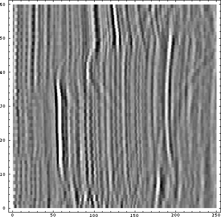 |
|
hilbertden
Figure 7 The Hilbert transform of the traces seen in Figure 6. | 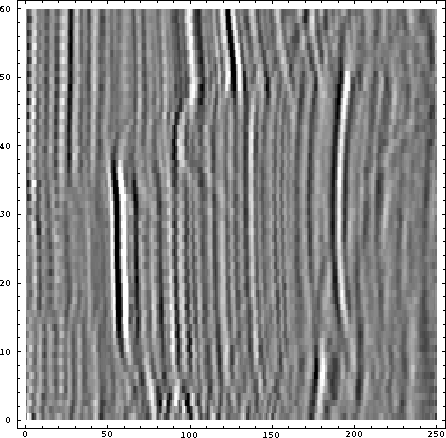 |
The envelope of the set of original traces may be generated using the square-root of the sums of the squares of the the corresponding samples in the original and transformed traces. The code to produce the envelope follows:
b = Map[Hilbert,a];
env=Sqrt[a^2+b^2];
The Hilbert transform routine in provided in the Appendix.
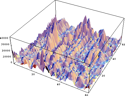
Figure 8 shows the ListDensityPlot display of the envelope trace. Figure 9 shows the data plotted with the ListPlot3D routine, subsampled in time. The 3-D plot gives a better idea of the variations of the envelope values.
|
envden
Figure 8 Density Plot of the envelope of the traces in Figure 6. | 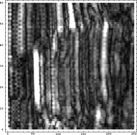 |
 |
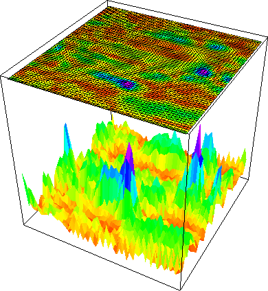
A combination of Figures 8 and 9 may be created using a three-D plot with a shadow display. Figure 10 shows such a plot. Notice that the plot is rotated with respect to Figure 9, and that the grid on the shadow portion of the plot hides much of the detail there. The grid on the shadow is the result of a bug in the shadow-graphics package. The black and white display of these data is much less effective than a color display.
 |
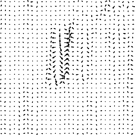
An interesting alternative to the separate trace displays in Figures 6 and 7 is the vector plot in Figure 11. This display allows the amplitude and a combination of the original and Hilbert-transformed traces to be displayed on one plot. These data have been subsampled in both time and space to allow a less cluttered plot.
 |
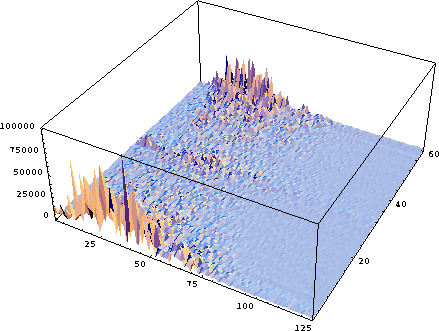
Another similar set of displays involves showing the two-D Fourier transforms of seismic data. The Fourier transform of the data in Figure 6 is shown in Figures 12, 13, and 14, displaying the real part, the imaginary part, and the absolute value of the transformed data. Figure 15 shows a three-D display of the data in Figure 14.
|
rs
Figure 12 The real part of the 2-D Fourier-transformed data. | 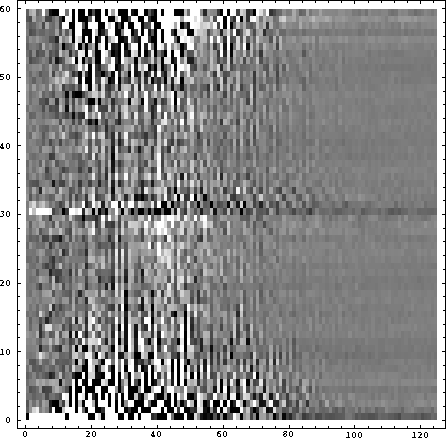 |
|
imag
Figure 13 The imaginary part of the 2-D Fourier-transformed data. | 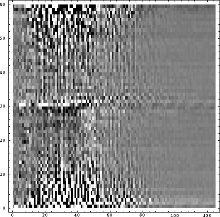 |
|
abs
Figure 14 The absolute values of the 2-D Fourier-transformed data. | 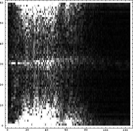 |
 |
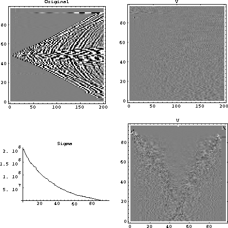
A final example shows the singular value decomposition of a seismic file. In this case a simple line plot has been mixed with the density plots of the original file and the U and V matrices.
 |