

Next: Synthetic data example
Up: Ji: Interpolation
Previous: Real data
For regridding irregularly sampled traces, the dip picking stage is the same
as the case of regularly sampled traces because slant stack works
in both cases.
We cannot use the simple Z-transform technique, however, to simulate
the prediction error filter for irregularly sampled case.
The filtering operation in a continuous signal is a convolution as follows:
|  |
(1) |
where y(t) is an filtered output, x(t) is an input and f(t) is a filter.
In the case of a discrete signal,
the integral operator can be approximated by summation operator as follows
|  |
(2) |
If discrete points are uniformly sampled,  is always same
so that it can be dropped.
But for irregularly sampled signal, the
  must be considered
in the convolution formula because it will vary with sampling
intervals.
If we write a filtering operation as a form of matrix multiplication,
the matrix which corresponds to this operation
will have a structure as shown below.
![\begin{displaymath}
\left[
\begin{array}
{c}
y_1\\ y_2\\ y_3\\ y_4\\ y_5\\ \end{...
...gin{array}
{c}
x_1\\ x_2\\ x_3\\ x_4\\ x_5\\ \end{array}\right]\end{displaymath}](img12.gif)
where  represent offset interval between i th trace and
i+1 th trace and
  represent the interval of regularly sampled
traces which is used to generate the prediction error filter.
The operation described above look like a nonstationary filtering operation.
But, the filter itself does not change and the change during the convolution
is the sampling point on the filter.
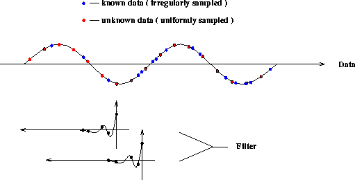
Each row of the matrix represents the same filter but the different
sampling points as explained in Figure
 ![[*]](http://sepwww.stanford.edu/latex2html/cross_ref_motif.gif) .
Figure
.
Figure ![[*]](http://sepwww.stanford.edu/latex2html/cross_ref_motif.gif) schematically shows this filtering operation.
At each position of the filter shifted to convolve with the irregularly
sampled data, all coefficients of the filter should be recalculated
from the spectrum of the filter.
Here, I make a spectrum by FFT for the prediction error filter
simulated as in the first section,
and sample at points where the filter meets the irregularly sampled data
points during the convolution.
Figure
schematically shows this filtering operation.
At each position of the filter shifted to convolve with the irregularly
sampled data, all coefficients of the filter should be recalculated
from the spectrum of the filter.
Here, I make a spectrum by FFT for the prediction error filter
simulated as in the first section,
and sample at points where the filter meets the irregularly sampled data
points during the convolution.
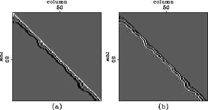
Figure ![[*]](http://sepwww.stanford.edu/latex2html/cross_ref_motif.gif) shows an example of the real and imaginary parts of the matrix
for filtering on irregularly sampled grid for a frequency.
irrgrim
shows an example of the real and imaginary parts of the matrix
for filtering on irregularly sampled grid for a frequency.
irrgrim
Figure 6 The convolution of an irregularly sampled data with a filter which is continuous.
 nsflt
nsflt
Figure 7 (a) Real component of the filter for the frequency of
an half of the Nyquist.
(b) Imaginary component of the filter for the frequency of
an half of the Nyquist.


Next: Synthetic data example
Up: Ji: Interpolation
Previous: Real data
Stanford Exploration Project
11/18/1997
![\begin{displaymath}
\left[
\begin{array}
{c}
y_1\\ y_2\\ y_3\\ y_4\\ y_5\\ \end{...
...gin{array}
{c}
x_1\\ x_2\\ x_3\\ x_4\\ x_5\\ \end{array}\right]\end{displaymath}](img12.gif)
![[*]](http://sepwww.stanford.edu/latex2html/cross_ref_motif.gif) .
Figure
.
Figure ![[*]](http://sepwww.stanford.edu/latex2html/cross_ref_motif.gif) schematically shows this filtering operation.
At each position of the filter shifted to convolve with the irregularly
sampled data, all coefficients of the filter should be recalculated
from the spectrum of the filter.
Here, I make a spectrum by FFT for the prediction error filter
simulated as in the first section,
and sample at points where the filter meets the irregularly sampled data
points during the convolution.
Figure
schematically shows this filtering operation.
At each position of the filter shifted to convolve with the irregularly
sampled data, all coefficients of the filter should be recalculated
from the spectrum of the filter.
Here, I make a spectrum by FFT for the prediction error filter
simulated as in the first section,
and sample at points where the filter meets the irregularly sampled data
points during the convolution.
Figure ![[*]](http://sepwww.stanford.edu/latex2html/cross_ref_motif.gif) shows an example of the real and imaginary parts of the matrix
for filtering on irregularly sampled grid for a frequency.
shows an example of the real and imaginary parts of the matrix
for filtering on irregularly sampled grid for a frequency.

