 |
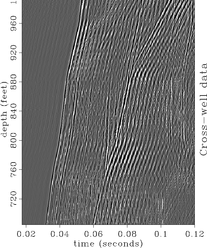
Figure 5 Cross-well data set before decimation. The trace separation is 1 foot.
![[*]](http://sepwww.stanford.edu/latex2html/cross_ref_motif.gif) ) consists of
316 traces, each containing 512 time samples. The traces are 1 foot
apart and are sampled at 0.2 ms. The shot was at 540 foot depth.
In order to test the interpolation algorithm,
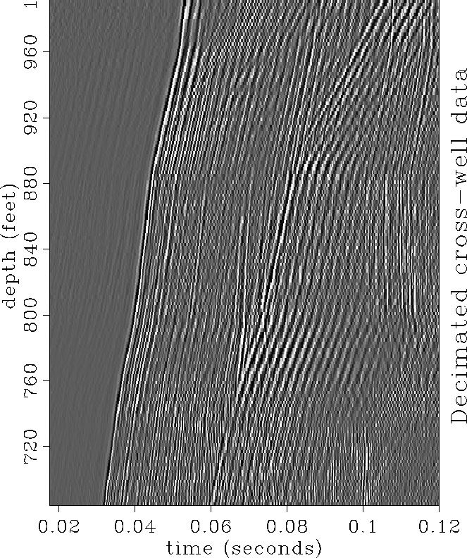
the data set was decimated by removing every other trace (Figure
) consists of
316 traces, each containing 512 time samples. The traces are 1 foot
apart and are sampled at 0.2 ms. The shot was at 540 foot depth.
In order to test the interpolation algorithm,
the data set was decimated by removing every other trace (Figure ![[*]](http://sepwww.stanford.edu/latex2html/cross_ref_motif.gif) ).
This spatially aliases the data and gives it a rougher checkerboard appearance.
A plot of the spectrum (Figure
).
This spatially aliases the data and gives it a rougher checkerboard appearance.
A plot of the spectrum (Figure ![[*]](http://sepwww.stanford.edu/latex2html/cross_ref_motif.gif) ) clearly shows the aliased
energy.
) clearly shows the aliased
energy.
 |
 |
 |
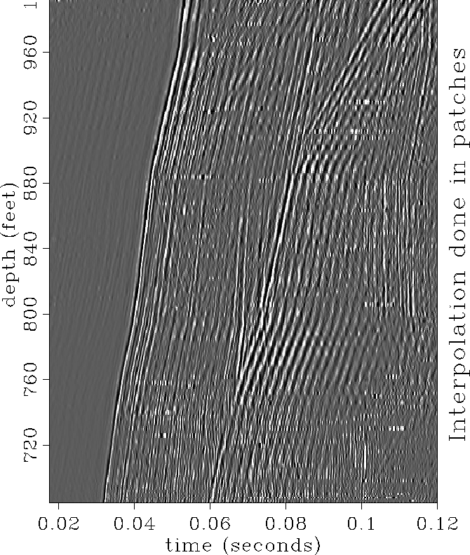
This data set is nonstationary. In order to perform the interpolation I must apply the algorithm to small windows of data and then piece these back together. This is done by the program Pstri() (Appendix). The data set is split up into 2048 overlapping windows. The shaping filter is calculated and applied in each window. The interpolated windows are then patched back together with triangular weights on each window.
The result of the interpolation is presented in Figure ![[*]](http://sepwww.stanford.edu/latex2html/cross_ref_motif.gif) .
This compares quite well to Figure
.
This compares quite well to Figure ![[*]](http://sepwww.stanford.edu/latex2html/cross_ref_motif.gif) . The events are now
much smoother and more continuos than in Figure
. The events are now
much smoother and more continuos than in Figure ![[*]](http://sepwww.stanford.edu/latex2html/cross_ref_motif.gif) . The
higher amplitude events are reconstructed better than the weaker
events.
. The
higher amplitude events are reconstructed better than the weaker
events.
There are artifacts in
the interpolation that I have not been able to removing yet. The
most distracting artifacts are the oscillations at various points
in the interpolated data (such as at depth=740', t=0.11s). These are due
to the aliasing of the shaping filter. Median filtering the
shaping filter is unsuccessful in removing these artifacts because
the shaping filter varies too much in each window. Increasing
the number of windows does reduce these artifacts. Some of the fainter
steeply dipping tube wave arrivals visible late in the section at depth=700'
to depth=800' in Figure ![[*]](http://sepwww.stanford.edu/latex2html/cross_ref_motif.gif) have been removed
by the interpolation (Figure
have been removed
by the interpolation (Figure ![[*]](http://sepwww.stanford.edu/latex2html/cross_ref_motif.gif) ). The tube waves arriving at
earlier times have also been attenuated. The algorithm has difficulty
reconstructing these arrivals because they are high frequency and relatively
low amplitude. Although it is often desirable to remove tube waves from
cross-well data, that is not the goal of interpolation.
). The tube waves arriving at
earlier times have also been attenuated. The algorithm has difficulty
reconstructing these arrivals because they are high frequency and relatively
low amplitude. Although it is often desirable to remove tube waves from
cross-well data, that is not the goal of interpolation.
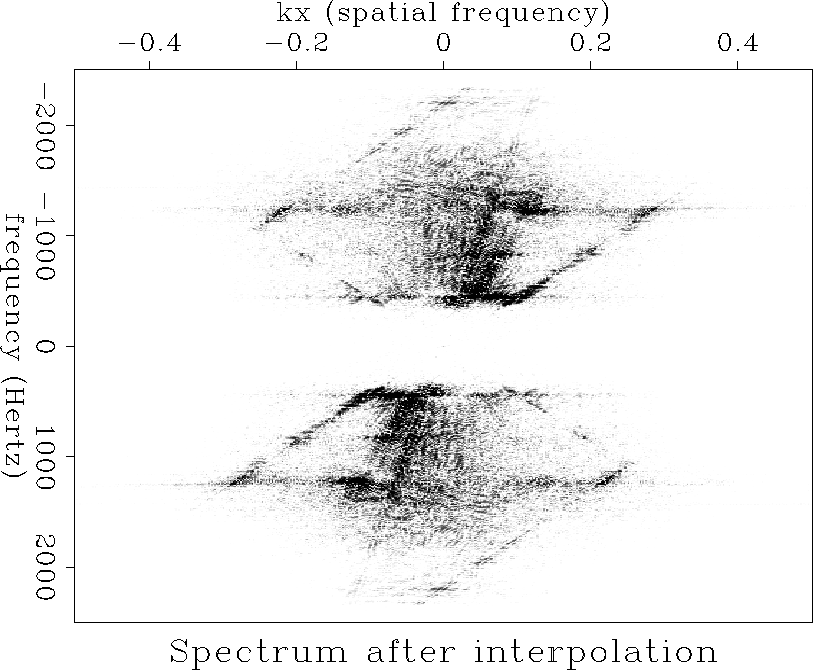
The spectrum of the interpolated cross-well data (Figure ![[*]](http://sepwww.stanford.edu/latex2html/cross_ref_motif.gif) ) shows
that most of the aliased energy has been removed.
) shows
that most of the aliased energy has been removed.
Windowing the data gives rise to a whole set of parameter choices which effect the final quality of the interpolation. In general, increasing the number of windows in which the interpolation is done increases the quality of the interpolation.
I plan to experiment with the shaping filter design in order to eliminate the artifacts due to filter aliasing. Since the effect of the filter aliasing is distinctive, it seems likely that it could be eliminated.
 |
 |