


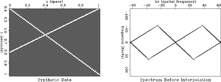
Figure ![[*]](http://sepwww.stanford.edu/latex2html/cross_ref_motif.gif) shows two crossing events and their amplitude spectra.
The steeply dipping event is aliased in space.
The shaping filter used to reconstruct the HF from the LF is shown in
Figure . This filter is convolved
with the cubed LF data on the interpolated traces to create the final
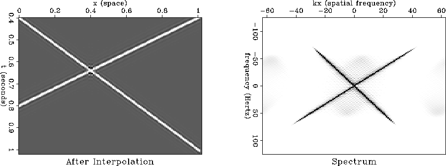
interpolated section (Figure ).
The prominent alias visible in
Figure has been removed.
However, the interpolation breaks down where the two events
cross. The break-down is seen as oscillations and distortions near the
crossing point in the time domain and as horizontal lines of
noise in the amplitude spectrum.
shows two crossing events and their amplitude spectra.
The steeply dipping event is aliased in space.
The shaping filter used to reconstruct the HF from the LF is shown in
Figure . This filter is convolved
with the cubed LF data on the interpolated traces to create the final
interpolated section (Figure ).
The prominent alias visible in
Figure has been removed.
However, the interpolation breaks down where the two events
cross. The break-down is seen as oscillations and distortions near the
crossing point in the time domain and as horizontal lines of
noise in the amplitude spectrum.
This distortion is due to the fact that the shaping filter is aliased in
space. Where the events are far apart, the shaping filter is very smooth.
Near the point where the events cross, the shaping filter gets
more complicated and varies rapidly in the spatial
direction (Figure ). The filter is calculated where both
the HF and LF are known and then interpolated to the trace locations
where the HF is unknown. Since the filter is aliased near crossing
events, distortions arise in the interpolation. In the previous examples
nearest neighbor interpolation was used to interpolate the shaping filter.
 |


|
crossshape
Figure 2 Shaping filter used to reconstruct the high-frequency data from the cubed low-frequency data. Notice the oscillations in the filter where the events cross. |  |
 |
The interpolation may be improved by median filtering the
shaping filter. The result of this
interpolation is presented in Figure . The result is much
more satisfying but the amplitude at the crossover may be a little too high
and there is still some noise visible in the frequency domain.
 |