The vectorizer operator

Using the partial derivatives defined by equations (15), (17), and (13), we can express equation (4) as a simple linear operation in the $\omega$-$\kappa_x$ domain:  

$${\bf u}(\kappa_x,z_0,\omega) \; = \; \mbox{\boldmath $\stack... ...im}{\kappa}$}(\kappa_x,z_0,\omega)\; \phi(\kappa_x,z_0,\omega),$$ (18)

where $\mbox{\boldmath$\stackrel{\sim}{\kappa}$}$ is the vectorizer operator, whose components are

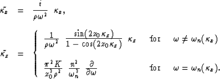$$\begin{eqnarray} \tilde{\kappa_x} & =& {i \over \rho \omega^2} \;\; \kappa_x, \\... ...box{for} & \;\; {\omega = \omega_n(\kappa_x).} \end{array} \right.\end{eqnarray}$$ (19) (20) (21)

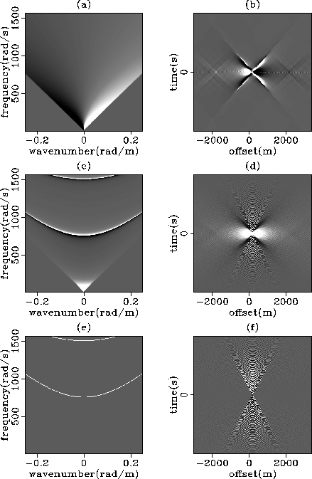
The horizontal and vertical components of the operator represented in equations (19) and (21), are illustrated in Figure  in both the frequency-wavenumber and the space-time domains. It is important to realize that while Figures -a and -c multiply the Fourier-transformed pressure field, -e multiplies the frequency-derivative of the same transformed field. Therefore, while -b and -d should be convolved with the pressure field, -f should be convolved with the time-scaled pressure field (which is, in practice, equivalent to convolving it with the wavefield corrected for 2-D divergence). Only the non-zero parts of the operator are represented in the figure, that is, the imaginary parts in -a and -f and the real parts in the other four images.

 

operator
Figure 1 Wavefield vectorizer operator. (a) $\tilde{\kappa_x}$ in $\omega$-$\kappa_x$domain. (b) $\tilde{\kappa_x}$ in x-t domain. (c) $\tilde{\kappa_z}$in $\omega$-$\kappa_x$ domain (for $\omega \neq \omega_n(\kappa_x)$). (d) $\tilde{\kappa_z}$ in x-t domain (for $\omega \neq \omega_n(\kappa_x)$). (e) $\tilde{\kappa_z}$ in $\omega$-$\kappa_x$ domain (for $\omega = \omega_n(\kappa_x)$). (f) $\tilde{\kappa_z}$ in x-t domain (for $\omega \neq \omega_n(\kappa_x)$).

It is interesting to observe that the impulse response of $\tilde{\kappa_x}$in the space-time domain clearly resembles a second derivative in time and a first derivative in space. Inverse theory tells us that the first approximation to the inverse is the conjugate operator, and in this case we find that the double time integration coming from the $1/\omega^2$term resembles a second time derivative in the time domain.