


We know how to determine the image of a reflector's location on a migrated
section. This location, of course, depends on the choice of the continuation
velocity vc. Being independent of a weight function ![]() ,
the location of caustics in the
x,z-plane is determined by the system of equations
,
the location of caustics in the
x,z-plane is determined by the system of equations
| |
(102) |
| |
(103) |
If at some velocity vc = vex the caustic and the image cross each other
at a special point ![]() , we call this the extremal velocity vex. Usually
we have a continuous interval of extremal velocities:
, we call this the extremal velocity vex. Usually
we have a continuous interval of extremal velocities: ![]() .Typically for each
.Typically for each ![]() one can observe two or more
special points. For some value vex = v*ex called the true extremal
velocity, these special points unify in one point that appears as a
bright spot.
one can observe two or more
special points. For some value vex = v*ex called the true extremal
velocity, these special points unify in one point that appears as a
bright spot.
Example: If the true model represents a homogeneous medium with velocity v and a planar reflector at depth h, the location of the reflector's image after CSP-migration is described by the system of equations (see Chapter 7):
 |
||
To find the location of caustics, we substitute
![]() and
and ![]() .into system equations (102) and (103).
So we have the system of equations
.into system equations (102) and (103).
So we have the system of equations
If for some ![]() and r we have
and r we have ![]() and
and ![]() , then the reflector's image contains the special point
, then the reflector's image contains the special point ![]() .Calculations show that at vc < v there is no special point on the image.
At
.Calculations show that at vc < v there is no special point on the image.
At ![]() we have two symmetrical special points which merge
together into the one bright point when
we have two symmetrical special points which merge
together into the one bright point when ![]() (as shown
in Figure
(as shown
in Figure ![[*]](http://sepwww.stanford.edu/latex2html/cross_ref_motif.gif) ).
).
Instead of a complete investigation of the situation, we can choose some particular ray of the eikonal ![]() .It is not difficult to determine the meaning of
.It is not difficult to determine the meaning of ![]() for the given velocity v=vc and the point
for the given velocity v=vc and the point ![]() belonging to the image and the ray
belonging to the image and the ray ![]() ; we can easily check condition (103).
Let us again consider CSP-migration with the true model containing a curved
reflector in a homogeneous medium (Figure , solid line). Let us
choose the ray
; we can easily check condition (103).
Let us again consider CSP-migration with the true model containing a curved
reflector in a homogeneous medium (Figure , solid line). Let us
choose the ray ![]() which approaches the surface
which approaches the surface ![]() vertically.
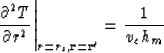
This ray is connected with a stationary point rs of the function
vertically.
This ray is connected with a stationary point rs of the function ![]() :
:
![]()
| |
(104) |
 |
(105) |
The point ![]() belongs to a caustic if
belongs to a caustic if
| |
(106) |
| |
(107) |
Combining (106) and (107) we receive
| |
(108) |
)
| |
(109) |
As for ![]() we can use standard techniques based on the continuation of wave front curvatures along the ray. We shall omit all these calculations and give the final result:
we can use standard techniques based on the continuation of wave front curvatures along the ray. We shall omit all these calculations and give the final result:
| |
(110) |
| |
(111) |
| |
(112) |
If the point ![]() is stationary for the reflector (
is stationary for the reflector (![]() ), then
), then
| |
(113) |
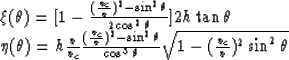
If the reflector is planar and horizontal (k=0 and ![]() ), then
), then
| |
(114) |
| vex = v | (115) |
Is this velocity vex the true extremal velocity? It is in all particular situations expressed by formulas (112) - (115).
In the zero offset case for arbitrary rays
![]()
![]()
In the common mid-point case travel-time curves for a point reflector and for a flat reflector are the same. It means that in this situation vex=v.