Residual moveout-based wave-equation migration velocity analysis in 3-D

2-D Theory Review

We start from the `classical' maximum-stack-power objective function

$$J(s) = \frac{1}{2} \sum_{x}\sum_{z} {\left[ \sum_{\gamma} \; I(z,\gamma,x;s) \right]}^2,$$ (1)

where $s$ is the model slowness, and $I(z,\gamma,x;s)$ is the prestack image (ADCIGs) migrated with $s$ .

Objective functions defined this way are prone to cycle-skipping (Symes, 2008). To tackle this issue, we approximate objective function 1 with the following one:

$$J(\rho(s)) = \frac{1}{2} \sum_{x}\sum_{z} {\left[ \sum_{\gamma} \; I(z+\rho\tan^2{\gamma},\gamma,x;s_0) \right]}^2,$$ (2)

in which $s$ is the model slowness, $I(z,\gamma,x;s_0)$ is the prestack image migrated with some initial slowness $s_{0}$ , and $\rho\tan^2{\gamma}$ is the residual moveout (RMO) function we choose to characterize the kinematic difference (Biondi and Symes, 2004) between $I(s)$    and $I(s_0)$ .

The meaning of equation 2 can be easily explained. As the model changes from $s_0$ to $s$ , it leads to the change of the image kinematics between $I(s_0)$    and $I(s)$ , where the differences are characterized by the moveout parameter $\rho$ . Since $I(s)$ will be kinematically the same as $I(s_0)$ being applied moveout $\rho(s)$ , if we substitute the former image ($I(s)$ ) with the latter one, we transit from equation 1 to equation 2. Notice that the new objective function is expressed as a function of only the moveout parameter $\rho$ , while the $\rho$ parameter is then related to the model slowness $s$ .

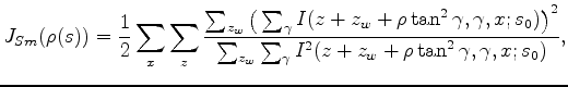
Furthermore, notice that equation 2 weights the strong-amplitude events more heavily. To make the gradient independent from the strength of reflectors, we further replace 2 with the following semblance objective function:

$$J_{Sm}(\rho(s)) = \frac{1}{2} \sum_{x}\sum_{z} \frac{\sum_{z_w} \... ...)\big)^2}{\sum_{z_w} \sum_{\gamma} I^2(z+z_w+\rho\tan^2{\gamma},\gamma,x;s_0)},$$ (3)

where $z_w$ is a local averaging window of length $L$ along the depth axis. For the rest of the paper, the summation interval of $z_w$ is always $[-L/2,L/2]$ ; thus we can safely omit the summation bounds for concise notation.

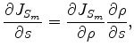
We will use gradient-based methods to solve this optimization problem. The gradient given by the objective function 3 is

$$\frac{\partial{J_{S_{m}}}}{\partial{s}} = \frac{\partial{J_{S_{m}}}}{\partial{\rho}} \frac{\partial{\rho}}{\partial{s}},$$ (4)

where ${\partial{J_{S_{m}}}}/{\partial{\rho}}$ can be easily calculated by taking the derivative along the $\rho$ axis of the semblance panel $S_{m}$ .

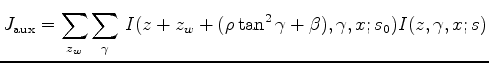
To evaluate the derivative of the moveout parameter $\rho$ with respect to the slowness model $s$ , we define an auxiliary objective function in a fashion similar to the one employed by Luo and Schuster (1991) for cross-well travel-time tomography. The auxiliary objective function is defined for each image point ($z,x$ ) as:

$$J_{\mathrm{aux}} = \sum_{z_w} \sum_{\gamma} \, I(z+z_w+ (\rho \tan^2{\gamma} + \beta),\gamma,x;s_0)I(z,\gamma,x;s)$$ (5)

where $\beta$ is a simple vertical shift introduced to accommodate bulk shifts in the image introduced by variation in the migration velocity. Notice that the semblance in objective function 3 is independent of $\beta$ because a bulk shift does not affect the power of the stack; therefore we do not include $\beta$ in 3.

The explanation for equation 5 is as follows: The moveout parameters $\beta(s)$    and $\rho(s)$ are chosen to describe the kinematic difference between the initial image $I(z,\gamma,x;s_0)$ and the new image $I(z,\gamma,x;s)$ . In other words, if we apply the moveout to the initial image, the resulting image $I(z+(\rho \tan^2{\gamma} + \beta),\gamma,x;s_0)$ will be the same as the new image $I(z,\gamma,x;s)$ in terms of kinematics; this is indicated by a maximum of the cross-correlation between the two.

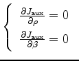
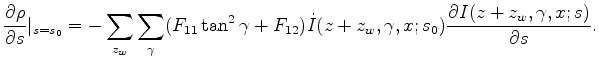
Given the auxiliary objective function 5, ${\partial{\rho}}/{\partial{s}}$ can be found using the rule of partial derivatives for implicit functions. We compute the gradient of 5 around the maximum at $s = s_0$ and $\rho = \beta = 0$ ; consequently

$$\renewedcommand{arraystretch}{1.5} \left\{ \begin{array}{c} \frac... ...\\ \frac{\partial{J_{\mathrm{aux}}}}{\partial \beta} = 0 \end{array} \, \right.$$ (6)

We differentiate equation 6 with respect to $s$ , which gives

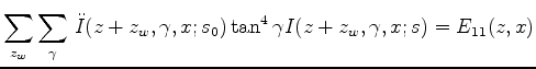
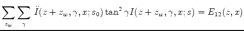
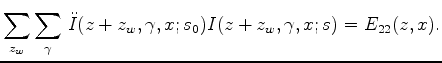
$$\renewedcommand{arraystretch}{1.5} \left[ \begin{array}{cc} \frac... ...{\partial{J_{\mathrm {aux}}}}{\partial{\beta}\partial{s}} \end{array} \right] .$$ (7)

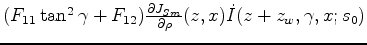
Now we need to invert a Jacobian to get ${\partial{\rho}}/{\partial{s}}$ . We denote $\dot{I}, \ddot{I}$ to be the first and second order $z$ derivatives of image $I$ , then define the following:

$$\frac{\partial^2{J_{\mathrm {aux}}}}{\partial{\rho}^2} = \sum_{z_w} \sum_{\gamma} \, \ddot{I}(z+z_w,\gamma,x;s_0) \tan^4{\gamma} I(z+z_w,\gamma,x;s) = E_{11}(z,x)$$

$$\frac{\partial^2{J_{\mathrm {aux}}}}{\partial{\rho}\partial{\beta}} = \sum_{z_w} \sum_{\gamma} \, \ddot{I}(z+z_w,\gamma,x;s_0) \tan^2{\gamma} I(z+z_w,\gamma,x;s) = E_{12}(z,x)$$

$$\frac{\partial^2{J_{\mathrm{aux}}}}{\partial{\beta^2}} = \sum_{z_w} \sum_{\gamma} \, \ddot{I}(z+z_w,\gamma,x;s_0) I(z+z_w,\gamma,x;s) = E_{22}(z,x).$$ (8)

Let the inverse of matrix $E$ be matrix $F$ :

$$F = \left[ \begin{array}{cc} F_{11} & F_{12} \\ F_{12} & F_{22} \... ...\begin{array}{cc} E_{11} & E_{12} \\ E_{12} & E_{22} \end{array} \right]^{-1}$$

Then

$$\frac{\partial{\rho}}{\partial{s}}\vert _{s=s_0} = -\sum_{z_w} \s... ... \dot{I}(z+z_w,\gamma,x;s_0) \frac{\partial{I(z+z_w,\gamma,x;s)}}{\partial{s}}.$$ (9)

Finally, we have the expression for the gradient

$$-\sum_{z_w} \sum_{\gamma} \sum_{z,x} \frac{\partial{I(z+z_w,\gamm... ...12}) \frac{\partial{J_{Sm}}}{\partial{\rho}}(z,x) \dot{I}(z+z_w,\gamma,x;s_0) .$$ (10)

The engineering translation of equation 10 is that first we compute the image perturbation $(F_{11}\tan^2{\gamma}+F_{12}) \frac{\partial{J_{Sm}}}{\partial{\rho}}(z,x) \dot{I}(z+z_w,\gamma,x;s_0)$ , then we backproject this perturbation to model slowness space using the tomography operator ${\partial{I(z+z_w,\gamma,x;s)}}/{\partial{s}}$ .

Since we can compute the gradient in equation 10, any gradient-based optimization method can be used to maximize the objective function defined in equation 3. Nonetheless, in terms of finding the step size, it is more expensive to evaluate equation 3 (which is an approximation of equation 1 purely based on kinematics) than to evaluate the original objective function 1. In our implementation we choose 1 as the maximization goal while using the search direction computed from equation 3.

Residual moveout-based wave-equation migration velocity analysis in 3-D