 |
 |
 |
 | Imaging with multiples using linearized full-wave inversion |  |
![[pdf]](icons/pdf.png) |
Next: Multiple imaging with towed
Up: Wong et al.: Linearized
Previous: Introduction
LFWI poses the imaging problem as an inversion problem by linearizing the wave-equation with respect to our model (
 ).
We define our model to be a weighted difference between the migration slowness (
).
We define our model to be a weighted difference between the migration slowness (
 ) and the true slowness (
 ):
):
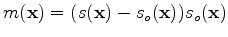 |
(1) |
Assuming that the earth behaves as a constant-density acoustic isotropic medium, we linearize the wave equation and apply the first-order Born approximation to get the following forward modeling equation:
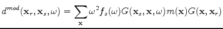 |
(2) |
where  represents the forward modeled data,
  is the temporal frequency,
is a function of the image point
is the temporal frequency,
is a function of the image point
 ,
,
 is the source waveform, and
 is the Green's function of the two-way acoustic constant-density wave equation over the migration slowness. Note that
  is actually
-dependent and is a function of
only.
It is important to point out that the adjoint of the forward-modeling operator is the migration operator:
is actually
-dependent and is a function of
only.
It is important to point out that the adjoint of the forward-modeling operator is the migration operator:
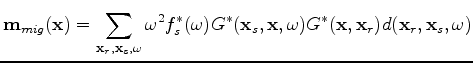 |
|
|
(3) |
The inversion problem is defined as minimizing the least-squares difference between the synthetic and the recorded data:
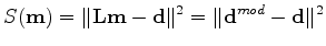 |
(4) |
where
 is the forward-modeling operator that corresponds to equation 2.
At first glance, equation 2 seems to only generate singly scattered events (e.g. Figure 1 a).
To clarify, the term scattering includes both diffraction and reflection. However, if we construct our propagator (
 ) using the two-way wave equation, equation 2 can actually generate multiply scattered events.
In figure 1 b, the ray path reflects off a salt flank and then the horizontal reflector.
If the sharp salt-flank boundary already exists in the migration velocity, then the scattering off the salt flank is automatically generated by the propagator (Green's function).
Figure 1 (c) and (d) shows two triply scattered events. Single circles (in purple) show scattering off the migration velocity, while double circles (in green) show scattering off the model
.
) using the two-way wave equation, equation 2 can actually generate multiply scattered events.
In figure 1 b, the ray path reflects off a salt flank and then the horizontal reflector.
If the sharp salt-flank boundary already exists in the migration velocity, then the scattering off the salt flank is automatically generated by the propagator (Green's function).
Figure 1 (c) and (d) shows two triply scattered events. Single circles (in purple) show scattering off the migration velocity, while double circles (in green) show scattering off the model
.
Subsections
|
|
|
|
| Imaging with multiples using linearized full-wave inversion | |
|
Next: Multiple imaging with towed
Up: Wong et al.: Linearized
Previous: Introduction
2012-05-10