|
|
|
|
VTI migration velocity analysis using RTM |
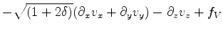
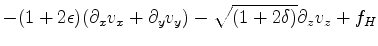
The first-order two-way VTI wave-equation can be derived from Hooke's law
and Newton's law using Thomson anisotropy parameters ( ,
,  ) and setting shear wave velocity
  (Duveneck et al., 2008). The first-order system reads as follows:
 is the density,
  is the velocity,
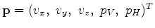
 is the particle velocity vector, and
  and
and  are
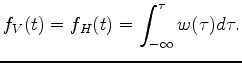
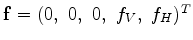
pressure in the vertical and horizontal directions, respectively. The source term
are
pressure in the vertical and horizontal directions, respectively. The source term
 and
and  are defined by the source wavelet
  as follows:
 ,
,
 and
and  ,
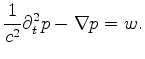
the first-order system 1 is equivalent to the familiar isotropic
acoustic second-order wave-equation:
,
the first-order system 1 is equivalent to the familiar isotropic
acoustic second-order wave-equation:
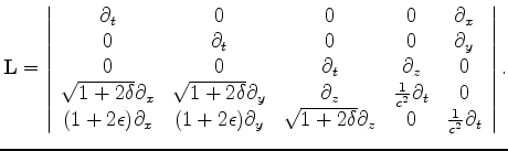
For simplicity, we can rewrite system 1 in a matrix-vector notation:
 ,
,
 ,
and
,
and
|
|
|
|
VTI migration velocity analysis using RTM |