VTI migration velocity analysis using RTM

Single parameter inversion

In this subsection, we invert for the anisotropic parameter $\epsilon$ alone. In this test, we model the synthetic data using very smooth $\epsilon$ (Figure 4(a)) and $\delta$ (Figure 4(b)) models as suggested by many field applications. To better constrain the inversion for $\epsilon$ , we also increase the maximum offset in the acquisition to 6 km.

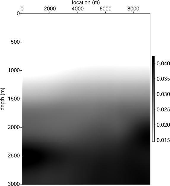
Compared with the true $\epsilon$ model, our initial $\epsilon$ model (Figure 5(a)) has negative perturbation of about 50% in the shallower part. Because a perfect velocity model is used in this case, the moveout at large angles is so small that it is almost undetectable to human eyes (Figure 5(b)). 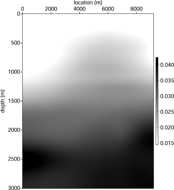However, our inversion scheme is very sensitive to the residual moveout and successfully updates the $\epsilon$ model in the correct direction. Figure 6 shows the inverted $\epsilon$ model and the corresponding angle-domain common-image gathers after 40 iterations. Comparing with the initial angle gathers (Figure 5(b)), we can see that the slightly curving events at large angles are flattened and the inverted $\epsilon$ model is closer to the true one.

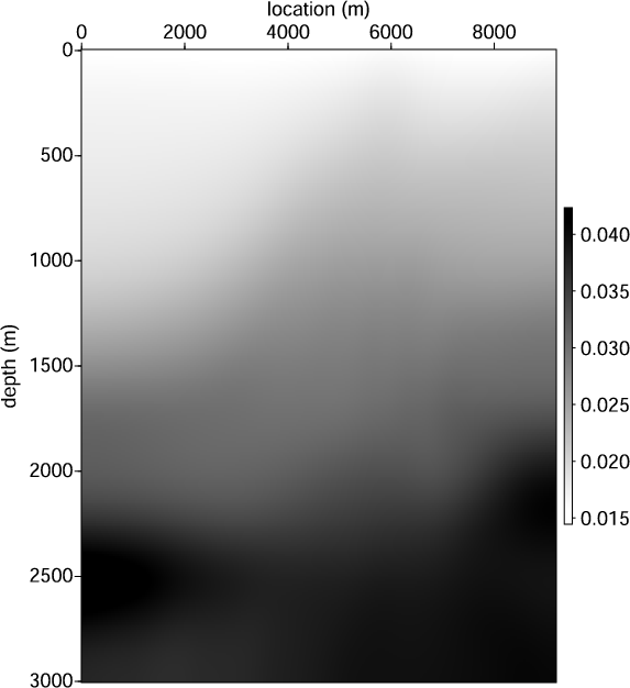
epssm,dltsm
Figure 4. (a) True $\epsilon$ model and (b) true $\delta$ model used to generate the synthetic data.

initeps,init-e-image
Figure 5. (a) Initial $\epsilon$ model and (b) initial angle-domain common-image gathers using initial $\epsilon$ model. Gathers are taken at every 10 common image point from $x=4$ km to $x=8$ km.

inveps,inv-e-image
Figure 6. (a) Inverted $\epsilon$ model and (b) final angle-domain common-image gathers using inverted $\epsilon$ model in (a). Compared with Figure 5(b), panel (b) shows more even energy across different angles. Gathers are taken at every 10 common image point from $x=4$ km to $x=8$ km.

VTI migration velocity analysis using RTM