|
|
|
|
VTI migration velocity analysis using RTM |
 model (Figure 2(a)) by a
very smooth
model (Figure 2(a)) by a
very smooth
 field, as shown in Figure 3(a).
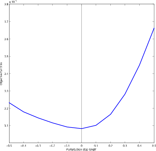
We change the perturbation from -50% to 50% of the true
model, and calculate the corresponding objective function respectively.
field, as shown in Figure 3(a).
We change the perturbation from -50% to 50% of the true
model, and calculate the corresponding objective function respectively.
Ideally, we'd like to choose an objective function that reaches a local minimum at the correct model and is quadratic around the correct model, so that a gradient-based inversion scheme is guaranteed to converge. Based on the results, we choose an angle domain objective function instead of the DSO objective function (Equation 15):
 is the Radon transform operator, and
  is the
derivative operator along the ray-parameter axis.
is the
derivative operator along the ray-parameter axis.
As shown in Figure 3(b), the angle-domain objective function
has a minimum at the correct epsilon model, and has a semi-quadratic shape
with respect to the model perturbation. Therefore, this objective function is
a good measure of the error in the anisotropic model.
Notice that the tilting effect toward negative
perturbation
is caused by the limited acquisition geometry. This effect is negligible for velocity
perturbation, because velocity has a first-order effect on the flatness of the
angle gather, while
's effect is second-order. We can increase the
acquisition offset to mitigate this tilting effect and help the inversion.

|
|---|
|
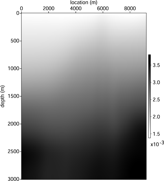
vtrue,ref
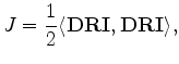
Figure 1. Smooth velocity model (a) in m/s and reflectivity model (b) used to generate the synthetic Born data. |
|
|

|
|---|
|
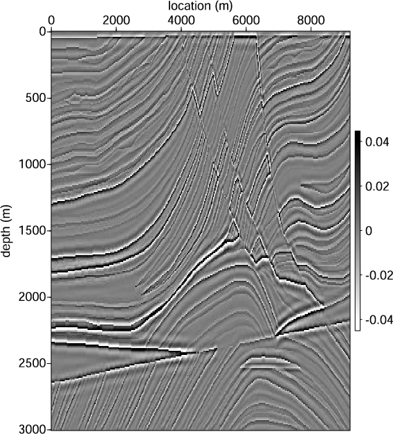
eps,del
Figure 2. The
model (a)
and  model (b) used to generate the synthetic Born data.
|
|
|
|
|---|
|
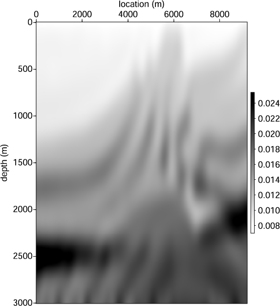
deltaeps,objcurve
Figure 3. (a) The
model to test the objective function. (b)
Objective function vs.
perturbation. The angle-domain objective function
45 has a minimum at the correct epsilon model, and has a semi-quadratic shape
with respect to the model perturbation.
|
|
|
|
|
|
|
VTI migration velocity analysis using RTM |