|
|
|
|
Image gather reconstruction using StOMP |
In RTM downward continuation based wave-equation imaging we have
a source
 and receiver wavefield
 , where
 is a given time and
  is a given shot. We
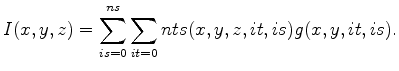
form our migrated image
is a given shot. We
form our migrated image  as
as
 |
(1) |
Several solutions to this problem have been proposed that attempt to extract information as a function of angle from the data. In this paper I focus on the family of methods that construct shift gathers by cross-correlation. The shift can be a function of space (Sava and Fomel, 2003) or time (Sava and Fomel, 2006), or both. In these cases the imaging condition takes the form of
 |
(2) |
 are how much the source and receiver wavefields have been
shifted in a given direction. Introducing these shift gathers poses two problems.
The first, and smaller of the problems, is that computational expense associated with
constructing these gathers, when going beyond a single shift
axis, is at least on the same order of magnitude as the propagation kernel.
The larger problem is the expansion of the volume size anywhere from 20-1000 fold,
means that the shift gathers must be stored a memory level further away from the processor,
often on disk, which is often several orders of magnitude more expensive to access.
Finding some way to reduce the volume size, and better still, the computational expense associated
with shift gather construction, can be highly beneficial. In order for compressive
sensing to be an appropriate way to reduce the volume size it is important
to consider the compressibility of seismic data.
are how much the source and receiver wavefields have been
shifted in a given direction. Introducing these shift gathers poses two problems.
The first, and smaller of the problems, is that computational expense associated with
constructing these gathers, when going beyond a single shift
axis, is at least on the same order of magnitude as the propagation kernel.
The larger problem is the expansion of the volume size anywhere from 20-1000 fold,
means that the shift gathers must be stored a memory level further away from the processor,
often on disk, which is often several orders of magnitude more expensive to access.
Finding some way to reduce the volume size, and better still, the computational expense associated
with shift gather construction, can be highly beneficial. In order for compressive
sensing to be an appropriate way to reduce the volume size it is important
to consider the compressibility of seismic data.
There is significant literature on compressing seismic data. Relatively low compression
ratios are achievable by compressing a trace. Significantly higher
compression ratios are achieved by multi-dimensional approaches. Generally, the best
results have used either multi-dimensional wavelets (Mallat, 1999) or its
successor curvelets (CandŹs and Donoho, 1999). Villasenor et al. (1996) showed that compression ratios
of 100:1 were achievable by compressing a 4-D volume (
 ). Further, Villasenor et al. (1996)
states
that the header information was the limiting factor in achieving even higher ratios.
). Further, Villasenor et al. (1996)
states
that the header information was the limiting factor in achieving even higher ratios.
Subsurface offset gathers potentially represent even higher, up to six, dimensional
data. To test compressibility, I used a 4-D volume ( ) of dimensions (32,32,400,64).
Figure 1 shows one of these subsurface offset gathers and its neighbors, note
the similarlity. Following Villasenor et al. (1996), I chose the 9/7 bi-orthonormal
transform (Antonini et al., 1992) used in JPEG compression.
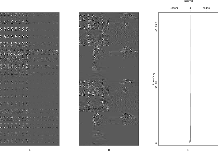
Figure 2 shows the resulting transform space and a histogram
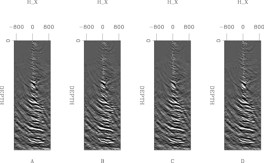
of the absolute values. I then used several different
thresholds throwing away 90%, 95%, 98%, and 99% of the data in the wavelet domain respectively.
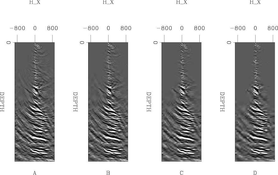
Figure 3
shows the result of transforming these thresholded volumes back into the space-domain.
The resulting images are near-perfect at 95% and potentially acceptable at 98%. This translates
into an acceptable compression ratio of approximately 30:1.
) of dimensions (32,32,400,64).
Figure 1 shows one of these subsurface offset gathers and its neighbors, note
the similarlity. Following Villasenor et al. (1996), I chose the 9/7 bi-orthonormal
transform (Antonini et al., 1992) used in JPEG compression.
Figure 2 shows the resulting transform space and a histogram
of the absolute values. I then used several different
thresholds throwing away 90%, 95%, 98%, and 99% of the data in the wavelet domain respectively.
Figure 3
shows the result of transforming these thresholded volumes back into the space-domain.
The resulting images are near-perfect at 95% and potentially acceptable at 98%. This translates
into an acceptable compression ratio of approximately 30:1.
|
|---|
|
raw
Figure 1. Five neighboring subsurface offset gathers. B and C are one midpoint in X before and after A. E is one midpoint in Y before A. Note the spatial similarity, which lends itself to compression. |
|
|
|
|---|
|
wavelet1
Figure 2. Panel A shows the wavelet domain representation of the 4-D volume used in this experiment. Panel B shows a zoom into a portion of the wavelet domain. Panel C shows a histogram of the wavelet domain values. Note how the vast majority of the values are nearly zero. |
|
|
|
|---|
|
offset
Figure 3. The result of zeroing the smallest values of the wavelet domain representation shown in Figure 2A. All four panels show the same subsurface offset gather shown in Figure 1. A shows the result of clipping 90% of the values; B, 95%; C, 98%; and D,99%. Note how the reconstructed gather is nearly identical up to a 98% clip. |
|
|
|
|
|
|
Image gather reconstruction using StOMP |