|
|
|
|
Fast automatic wave-equation migration velocity analysis using encoded simultaneous sources |
I apply the encoded simultaneous-source WEMVA on a truncated Marmousi model.
The data used for inversion are generated using prestack Born wavefield modeling (Tang, 2011; Stolt and Benson, 1986).
Hence the data only contain primary reflections and fit the theory perfectly.
I use one-way wavefield extrapolation to carry out the numerical experiments.
Since one-way wavefield extrapolation does not generate back scatterings, the velocity model used for Born modeling does
not need to be smooth.
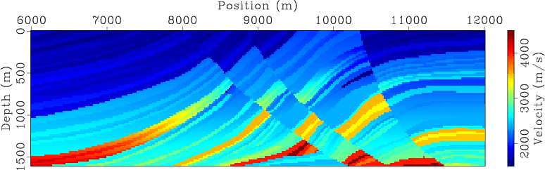
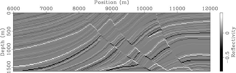
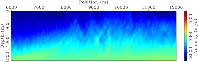
Figures 1(a) and 1(b) show the velocity model and reflectivity model used for Born modeling.
I use a Ricker wavelet with a dominant frequency of 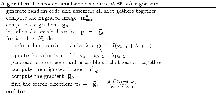 Hz as the source function for modeling. The source function is assumed
to be known in the subsequent inversion tests.
Hz as the source function for modeling. The source function is assumed
to be known in the subsequent inversion tests.
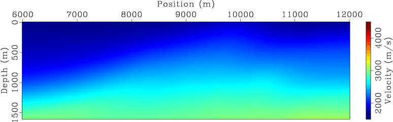
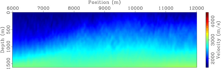
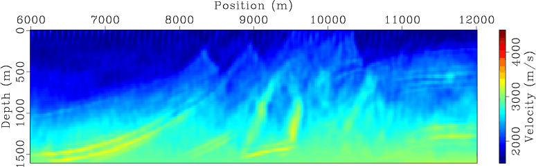
The initial velocity model used for inversion is shown in Figure 2. It is a smoothed version of the true velocity model (Figure 1(a)). The initial velocity model is accurate enough so that no cycle skipping occurs during inversion. The goal of the experiments shown here is to demonstrate that with an initial velocity model that guarantees the convergence of inversion, encoded simultaneous-source WEMVA produces similar inversion result as does conventional separate-source WEMVA, but with a significantly reduced computational cost. However, the convergence property using an initial velocity model far from the correct one still needs to be studied, and it remains an area for further investigation.
|
|---|
|
marm-vmod,marm-refl
Figure 1. The velocity model (a) and reflectivity model (b) used for Born wavefield modeling. |
|
|
|
|---|
|
marm-bvel
Figure 2. The initial velocity model. |
|
|
I test the inversion on data sets acquired using both land and marine acquisition geometries.
The data acquired from a land acquisition geometry contains ![]() shots ranging from
shots ranging from ![]() km to
km to ![]() km with a
km with a ![]() m sampling interval.
The receiver spread ranges from
m sampling interval.
The receiver spread ranges from ![]() km to
km to ![]() km and is fixed for all shots. The receiver sampling interval is
km and is fixed for all shots. The receiver sampling interval is ![]() m.
For the data acquired using a marine acquisition geometry, the
m.
For the data acquired using a marine acquisition geometry, the ![]() sources also range from
sources also range from ![]() km to
km to ![]() km and sampled at
km and sampled at ![]() m.
The minimum and maximum offsets for each shot is 0
and
m.
The minimum and maximum offsets for each shot is 0
and ![]() km. The receiver sampling interval is also
km. The receiver sampling interval is also ![]() m.
m.
I run inversion using both separate sources and encoded simultaneous sources after the same number of iterations. Figures 3 and 4 compare the WEMVA gradients at the first iteration for different methods and different acquisition geometries. Note the randomized crosstalk present in the simultaneous-source WEMVA gradients. Because I regenerate the random code at the beginning of each iteration, the crosstalk is expected to be incoherently stacked over iterations. Therefore, the impact of crosstalk will be mitigated.
|
|---|
|
marm-grad-separate,marm-grad-separate-marine
Figure 3. Gradient of separate-source WEMVA at the first iteration for (a) land acquisition geometry and (b) marine acquisition geometry. |
|
|
|
|---|
|
marm-grad,marm-grad-marine
Figure 4. Gradient of encoded simultaneous-source WEMVA at the first iteration for (a) land acquisition geometry and (b) marine acquisition geometry. |
|
|
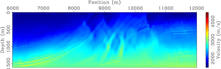
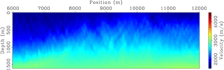
Figures 5 and 6 show the separate-source inversion results at different iterations for land and marine acquisition geometries, respectively. The velocity model has been successfully recovered in both cases. But inversion using land acquisition geometry produces a slightly better final inversion result (Figure 5(d)) than the one obtained using marine acquisition geometry (Figure 6(d)). This is because, for this particular example, the land acquisition geometry has wider offsets and hence gives better coverage to the model.
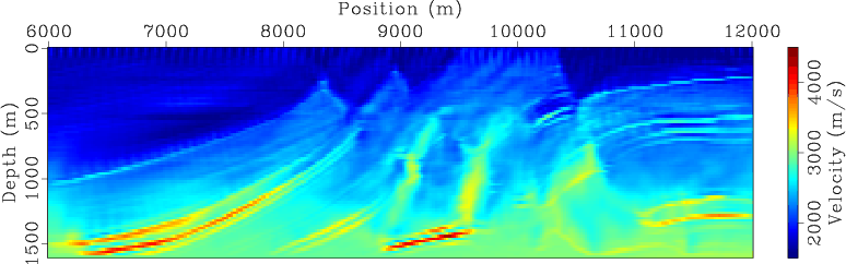
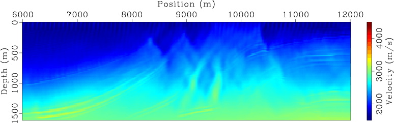
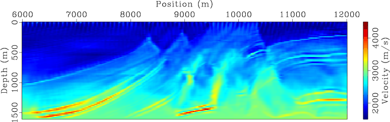
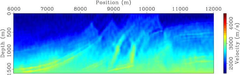
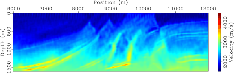
For comparison, Figures 7 and 8 present the encoded simultaneous-source inversion results for land and marine acquisition geometries, respectively. As expected, the inverted velocity model at early iterations (Figures 7(a) and 7(b) for land acquisition geometry and Figures 8(a) and 8(b) for marine acquisition geometry) have been strongly affected by the crosstalk artifacts in the gradients (Figure 4). As inversion proceeds, the crosstalk artifacts are destructively stacked, and hence the influence of crosstalk is decreasing over iterations. The final inversion results (Figures 7(d) and 8(d)) also successfully recover the velocity model. However, the encoded simultaneous-source WEMVA seems to be more sensitive to the model coverage, and the convergence of inversion using the data acquired with a marine geometry (Figure 8(d)) is considerably slower than that obtained using the data acquired from a land acquisition geometry (Figure 7(d)).


|
|---|
|
sinvt5,sinvt20,sinvt50,sinvt120
Figure 5. Separate-source WEMVA inversion result for land acquisition geometry at (a) |
|
|


|
|---|
|
sminvt5,sminvt20,sminvt50,sminvt120
Figure 6. Separate-source WEMVA inversion result for marine acquisition geometry at (a) |
|
|

|
|---|
|
invt5,invt20,invt50,invt120
Figure 7. Encoded simultaneous-source WEMVA inversion result for land acquisition geometry at (a) |
|
|

|
|---|
|
minvt5,minvt20,minvt50,minvt120
Figure 8. Encoded simultaneous-source WEMVA inversion result for marine acquisition geometry at (a) |
|
|
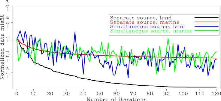
As a further comparison of the convergence, Figure 9 shows the data misfit (the objective function) obtained using different
methods and for different acquisition geometries. The data misfit curve for each case has been normalized with its value at the first iteration. Note that the data misfit
functions decrease monotonically for separate-source inversions. This is because the objective function ![]() is consistent over iterations,
and therefore the nonlinear conjugate gradient algorithm tries to minimize the same objective function over iterations.
In contrast, the data misfit functions for encoded simultaneous-source inversions fluctuate significantly, and they do not show monotonically decreasing behavior
as do separate-source inversions. This is because the random phase encoding function keeps changing at each iteration, and consequently the
objective function
is consistent over iterations,
and therefore the nonlinear conjugate gradient algorithm tries to minimize the same objective function over iterations.
In contrast, the data misfit functions for encoded simultaneous-source inversions fluctuate significantly, and they do not show monotonically decreasing behavior
as do separate-source inversions. This is because the random phase encoding function keeps changing at each iteration, and consequently the
objective function
![]() varies over iterations. The nonlinear conjugate gradient algorithm cannot guarantee the monotonic decrease of the objective function.
But the misfit functions do show an overall decreasing trend.
varies over iterations. The nonlinear conjugate gradient algorithm cannot guarantee the monotonic decrease of the objective function.
But the misfit functions do show an overall decreasing trend.
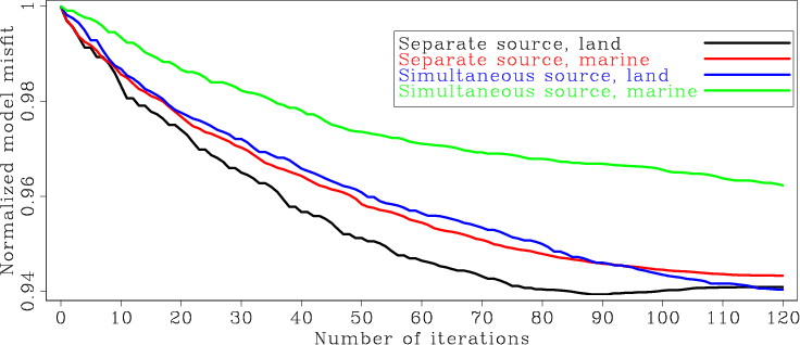
Since this is a synthetic-data example, the true velocity model is known. I calculate the model misfit in ![]() norm and the results are plotted in Figure 10.
It is interesting to note that although encoded simultaneous-source inversion does not show monotonic decrease of the data misfit, it does show monotonic decrease
of the model misfit, which suggests that the inversion is going in the correct direction. Also note that the model convergence of encoded simultaneous-source inversion
is slower than that of separate-source inversion. The difference seems to be insignificant for land acquisition geometries, where the receivers are fixed and the offsets are longer.
The difference for marine acquisition geometries, however, is much bigger. This is probably because the marine acquisition geometry used in this example has shorter offsets and
the data coverage is much less than the land acquisition geometry. The lack of data coverage may require more iterations to remove the crosstalk artifacts.
This speculation, however, still needs more investigation to verify.
norm and the results are plotted in Figure 10.
It is interesting to note that although encoded simultaneous-source inversion does not show monotonic decrease of the data misfit, it does show monotonic decrease
of the model misfit, which suggests that the inversion is going in the correct direction. Also note that the model convergence of encoded simultaneous-source inversion
is slower than that of separate-source inversion. The difference seems to be insignificant for land acquisition geometries, where the receivers are fixed and the offsets are longer.
The difference for marine acquisition geometries, however, is much bigger. This is probably because the marine acquisition geometry used in this example has shorter offsets and
the data coverage is much less than the land acquisition geometry. The lack of data coverage may require more iterations to remove the crosstalk artifacts.
This speculation, however, still needs more investigation to verify.
|
|---|
|
marm-dfit
Figure 9. Normalized data misfit as a function of iterations for different methods. |
|
|
|
|---|
|
marm-mfit
Figure 10. Normalized model misfit as a function of iterations for different methods. |
|
|
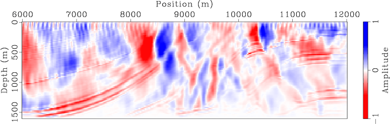
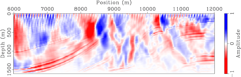
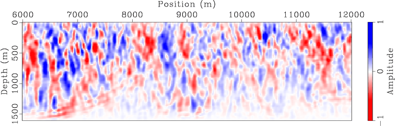
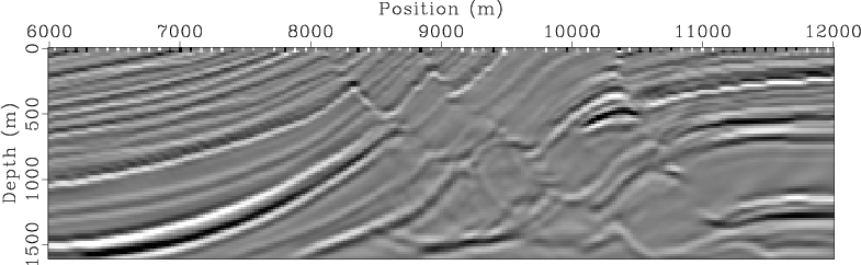
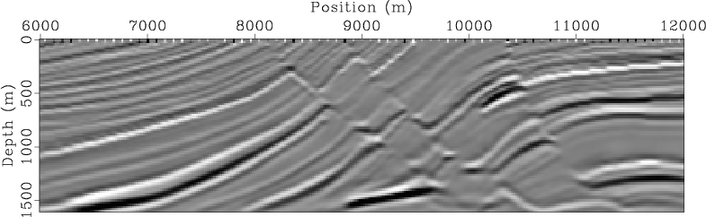
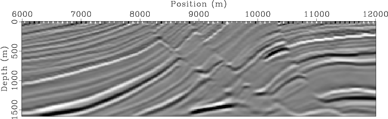
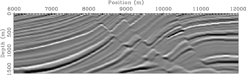
A final comparison is made among the images obtained using the inverted velocity model produced by different methods and for different acquisition geometries.
The initial images (Figure 11) show poor focusing due to the velocity errors. The updated images using velocities obtained
with separate sources (Figure 13) and encoded simultaneous sources (Figure 13) show
significantly improvements on image focusing and coherence. The updated images using both separate-source inversion and encoded simultaneous-source inversion
show very similar overall qualities, although separate-source inversion does produces slightly better images. But if we take the cost into account,
the encoded simultaneous-source inversion is about ![]() times faster than the separate-source inversion, which is a significant advantage.
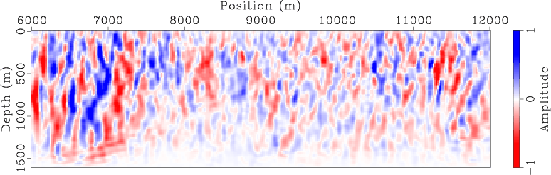
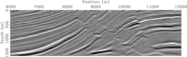
For comparison, Figure 14 presents images obtained using the true velocity model (Figure 1(a)).
times faster than the separate-source inversion, which is a significant advantage.
For comparison, Figure 14 presents images obtained using the true velocity model (Figure 1(a)).

|
|---|
|
bimg,bimg-marine
Figure 11. Image obtained using the initial velocity model (Figure 2) for (a) land acquisition geometry and (b) marine acquisition geometry. |
|
|
|
|---|
|
imag-invt-separate,imag-invt-separate-marine
Figure 12. Image obtained using the separate-source inverted velocity model for (a) land acquisition geometry and (b) marine acquisition geometry. |
|
|

|
|---|
|
imag-invt,imag-invt-marine
Figure 13. Image obtained using the encoded simultaneous-source inverted velocity model for (a) land acquisition geometry and (b) marine acquisition geometry. |
|
|

|
|---|
|
imag,imag-marine
Figure 14. Image obtained using the true velocity model (Figure 1(a)) for (a) land acquisition geometry and (b) marine acquisition geometry. |
|
|
|
|
|
|
Fast automatic wave-equation migration velocity analysis using encoded simultaneous sources |