Angle-domain illumination gathers by wave-equation-based methods

Subsurface-offset-domain image and illumination

Linearized modeling (Born modeling) from a prestack image parameterized as a function of subsurface offset can be described as follows:

$$d({\bf x}_r,{\bf x}_s,\omega) = \sum_{{\bf x}}\sum_{{\bf h}}L_{h}({\bf x},{\bf h},{\bf x}_r,{\bf x}_s,\omega)m_h({\bf x},{\bf h}),$$ (1)

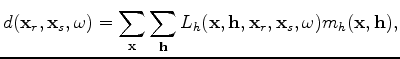where $d({\bf x}_r,{\bf x}_s,\omega)$ is the seismic data with a source located at ${\bf x}_s=(x_s,y_s,z_s=0)$ and a receiver located at ${\bf x}_r=(x_r,y_r,z_r=0)$ ; $\omega$ is the angular frequency; $m_h({\bf x},{\bf h})$ is the prestack image located at ${\bf x}=(x,y,z)$ for a half subsurface offset ${\bf h}=(h_x,h_y,h_z)$ ; $L_{h}$ is the sensitivity kernel defined as follows:

$$L_{h}({\bf x},{\bf h},{\bf x}_r,{\bf x}_s,\omega) = \omega^2f_s(\omega)G({\bf x}-{\bf h},{\bf x}_s,\omega)G({\bf x}+{\bf h},{\bf x}_r,\omega),$$ (2)

where $f_s(\omega)$ is the source signature, and $G({\bf x},{\bf x}_s,\omega)$ and $G({\bf x},{\bf x}_r,\omega)$ are the Green's functions connecting the source and receiver, respectively, to the image point ${\bf x}$ .

Reconstruction of the prestack image $m({\bf x},{\bf h})$ can be posed as an inverse problem by minimizing the following objective function defined in the data space:

$$F({\bf m}) = \frac{1}{2}\sum_{\omega}\sum_{{\bf x}_s}\sum_{{\bf x}_r}\vert W({\bf x}_r,{\bf x}_s)r({\bf x}_r,{\bf x}_s,\omega)\vert^2,$$ (3)

where $r({\bf x}_r,{\bf x}_s,\omega)=d({\bf x}_r,{\bf x}_s,\omega)-d_{\rm obs}({\bf x}_r,{\bf x}_s,\omega)$ is the data residual and $W({\bf x}_r,{\bf x}_s)$ is the acquisition mask operator, which contains unity values where we record data and zeros where we do not. The gradient of the objective function $F$ reads

$$I_{h}({\bf x},{\bf h}) = \sum_{\omega} \sum_{{\bf x}_s} \sum_{{\b... ...}^{*}({\bf x},{\bf h},{\bf x}_r,{\bf x}_s,\omega)r({\bf x}_r,{\bf x}_s,\omega),$$ (4)

where $^{*}$ denotes complex conjugation. Equation 4 is similar to the prestack shot-profile migration formula and it produces migrated reflectivity images defined in the subsurface offset domain (Rickett and Sava, 2002).

The Hessian can be obtained by taking the second-order derivatives of $F$ with respect to the model parameters as follows:

$$H_{h}({\bf x},{\bf x}',{\bf h},{\bf h}') =\sum_{\omega} \sum_{{\b... ...\bf x}_r,{\bf x}_s,\omega) L_{h}({\bf x}',{\bf h}',{\bf x}_r,{\bf x}_s,\omega).$$ (5)

When ${\bf x}={\bf x}'$ and ${\bf h}={\bf h}'$ , we obtain the diagonal elements of the Hessian operator

$$H_{h}({\bf x},{\bf h}) = \sum_{\omega}\sum_{{\bf x}_s}\sum_{{\bf ... ...x}_r,{\bf x}_s) \vert L_{h}({\bf x},{\bf h},{\bf x}_r,{\bf x}_s,\omega)\vert^2.$$ (6)

The diagonal of the Hessian is often known as the illumination map of the subsurface, it contains illumination contribution from both sources and receivers for a given acquisition configuration.

Angle-domain illumination gathers by wave-equation-based methods