Near-surface velocity estimation by weighted early-arrival waveform inversion

Data recorded with elastic wave equation

Next I estimate the the near-surface velocity using recorded data that is generated by the elastic wave equation. The synthetic P-wave velocity model used in this case is provided by Saudi Aramco. It simulates typical near-surface velocity encountered in Saudi Arabia. For elastic modeling, the density is obtained by the Gardner equation (Gardner et al., 1974). S-wave velocity is scaled from P-wave velocity. The model is $1600$ by $176$ grid in $x$ and $z$ , with $5$ m spacing in both directions. The acquisition geometry is also relatively simple. Receivers are on all the grid points on the surface, and there are $90$ shots with equal spacing of $80$ m. Inversion is done on a $10$ m spacing grid, which is coarser than the grid used for modeling. The major goal of acoustic inversion in this case is to see if waveform inversion can retrieve the velocity inversion layer.

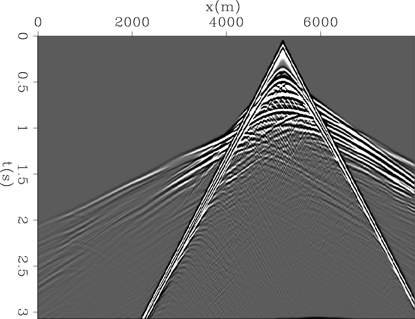
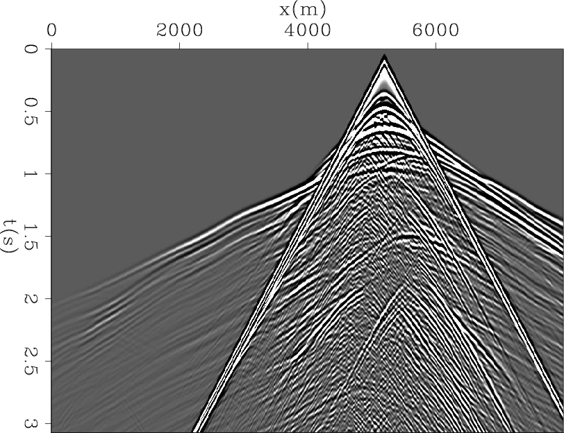
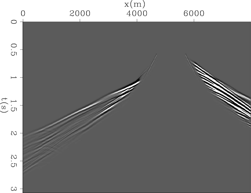
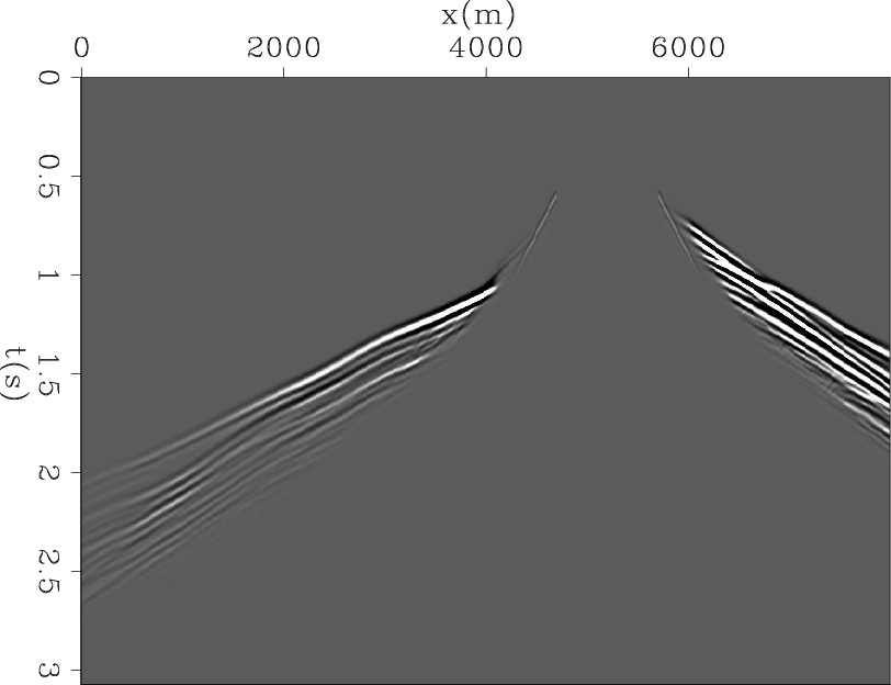
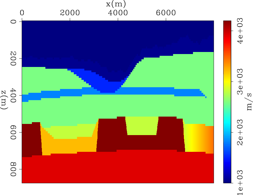
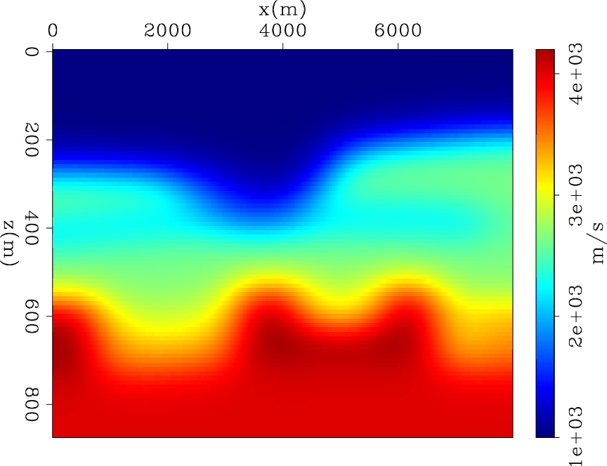
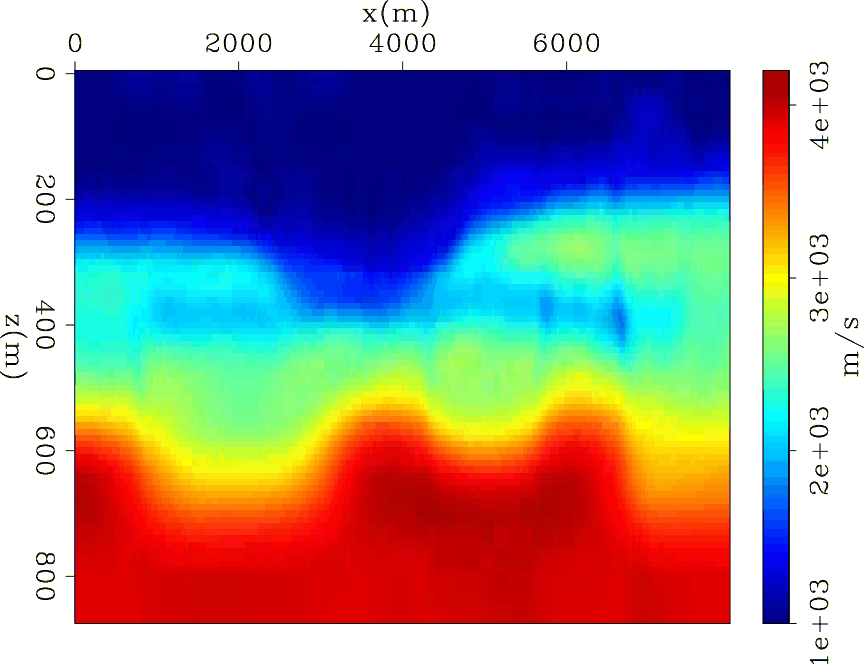
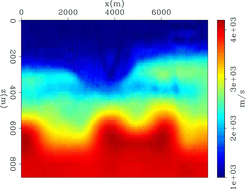
One shot gather from data with acoustic and elastic modeling is shown in figure 4; the left panel is the data with acoustic modeling, and the right panel is the data with elastic modeling. It can be seen that data from elastic modeling has some amplitude/phase difference and also some extra events that are converted waves. In this case, I scaled the amplitude of both shots to approximately the same level for display purposes. Figure 5 shows refraction events for the same shot. When I carefully mask out most of the converted waves, the remaining refraction events looks very similar in terms of kinematics; the difference at this point is likely to be caused by different distribution of P-wave and S-wave energy at different reflector boundaries. Figure 6 shows the true near-surface velocity and the starting velocity model; the starting velocity model is a smoothed version of true velocity model. The result of estimated velocity using proposed waveform inversion fitting goal are shown in figure 7. The top panel is the result of inverting acoustic data, whereas the bottom is the result of inverting elastic data. It can be seen that even with strong elastic effects in data, after excluding most converted waves, the weighted fitting goal was still able to recover the velocity inversion structure. Compared with inversion of acoustic data, there are some small shifts of reflector locations. This kind of shift is likely due to the very sharp velocity contrast immediately below the slow velocity.

This example shows that without the presence of most converted wave, acoustic inversion of elastic data can still obtain a decent velocity estimation result.

Arcd,Ercd
Figure 4. Shot gather generated by different modeling equations: a) shot generated by the acoustic wave equation b) the same shot generated by the elastic wave equation.

Arefrac,Erefrac
Figure 5. Refraction of the same shot generated by different modeling equations: a) refraction of shot generated by the acoustic wave equation b) refraction of same shot generated by the elastic wave equation.

veltrue,velstart
Figure 6. a) True near-surface velocity. b) Starting near-surface velocity model used for waveform inversion; the starting velocity model is a smoothed version of the true velocity model.

velinvArcd,velinvErcd
Figure 7. Estimated velocity using data from different modeling equations: a) estimated velocity using data generated by the acoustic wave equation. b) Estimated velocity using data generated by the elastic wave equation.

Near-surface velocity estimation by weighted early-arrival waveform inversion