Near-surface velocity estimation by weighted early-arrival waveform inversion

Data recorded with strong subsurface attenuation

Here I estimate near-surface velocity using recorded data with strong subsurface attenuation. The model is from Amoco-2.5D synthetic velocity model. The Q value is a scaled version of velocity to maintain consistency between structures. The velocity model is $600$ by $140$ grid in $x$ and $z$ , with $10$ m spacing in both directions. The acquisition geometry is relatively simple. Receivers are on all the grid points on the surface, there are $30$ shots with uniform spacing of $100$ m.

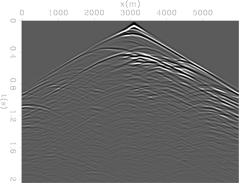
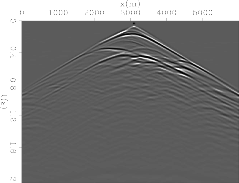
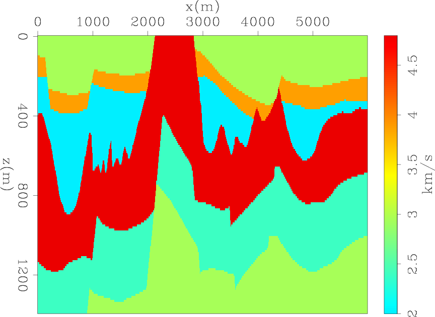
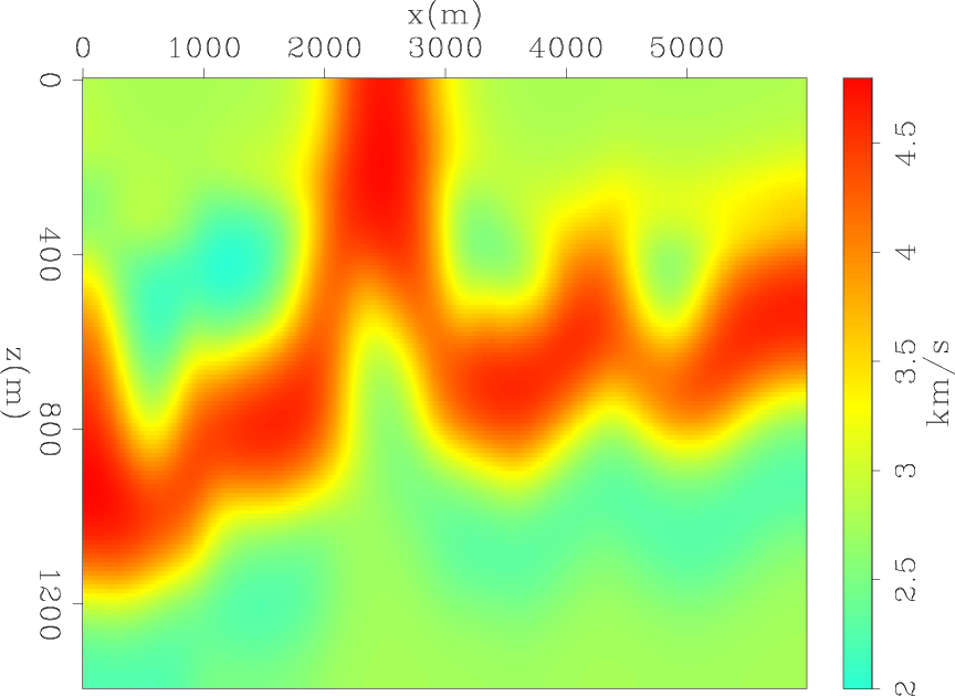
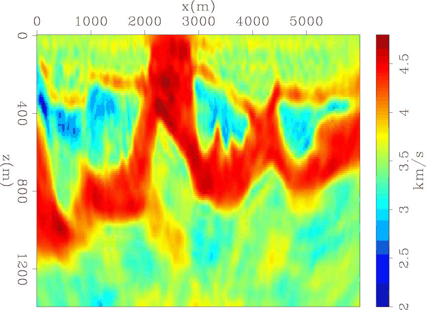
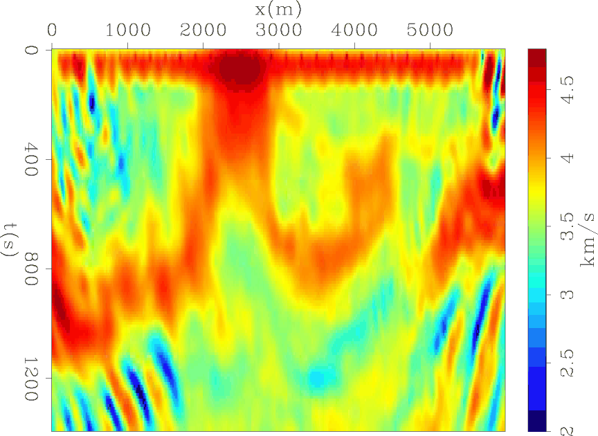
A shot gather at a single location from data is shown in figure 1; the left panel shows the data without attenuation, and the right panel shows the data with attenuation. It can be seen that the attenuated data has lower frequency content and much weaker amplitude. However, the kinematics of the data does not change much. Thus, in this case, phase information in the data is relatively insensitive to non-acoustic physics in the recorded data. Figure 2 shows the true near-surface velocity and starting velocity model. The results of estimated velocity using conventional waveform inversion fitting goals and weighted waveform inversion fitting goal are shown in figure 3. It can be seen that with strongly attenuated data, weighted waveform inversion is still able to recover the velocity model, while conventional fitting goal completely fails in this case. Since conventional waveform inversion use both phase and amplitude information in the recorded data, it tries to interpret weak amplitude as a result of a fast velocity layer at the surface. The new objective function, however, focuses more on phase information and partially ignores amplitude information to give a much better result.

nrmrcd,attenrcd
Figure 1. One synthetic shot with and without attenuation. Both panels have the same clip value. a) One shot generated by the acoustic wave equation. b) Same shot gather generated by the visco-acoustic wave equation with the amplitude of the entire shot gather scaled by a factor of ten.

attenveltrue,attenvelstart
Figure 2. a) True near-surface velocity. b) Starting near-surface velocity model used for waveform inversion.

velinvpropattenrcd,velinvconvattenrcd
Figure 3. Estimated velocity using different objective functions. a) Estimated velocity using the new objective function. b) Estimated velocity using the conventional objective function.

Near-surface velocity estimation by weighted early-arrival waveform inversion