|
|
|
|
Joint least-squares inversion of up- and down-going signal for ocean bottom data sets |
where
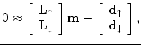 and
and
![]() are modeling operators that produce up-going data (
are modeling operators that produce up-going data (
![]() ) and down-going data (
) and down-going data (
![]() ) from the model space (
) from the model space (![]() ). The up- and down-going operators can be defined in many ways with varying levels of difficulty and practicality. We use the adjoint of the acoustic reverse time migration (RTM) operator to formulate
and
). The up- and down-going operators can be defined in many ways with varying levels of difficulty and practicality. We use the adjoint of the acoustic reverse time migration (RTM) operator to formulate
and
![]() . Two modified computational grids are used to forward model the lowest order of up- and down-going signals, namely the primary and the receiver ghost. The formulation of the modeling and its adjoint (RTM) operator is summarized in Figure 2 and Figure 3.
. Two modified computational grids are used to forward model the lowest order of up- and down-going signals, namely the primary and the receiver ghost. The formulation of the modeling and its adjoint (RTM) operator is summarized in Figure 2 and Figure 3.
|
|---|
|
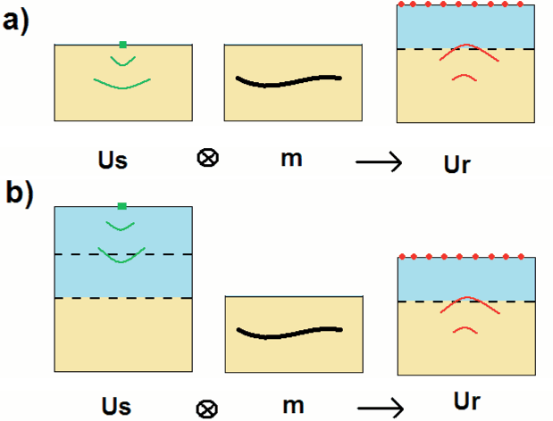
forward
Figure 2. Forward modeling of (a) primary-only and (b) mirror-only data. The algorithm involves cross-correlating the source wavefield ( |
|
|
|
|---|
|
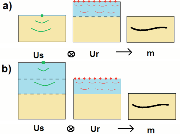
reverse
Figure 3. RTM of (a) primary-only and (b) mirror-only data. The algorithm involves cross-correlating the source wave field ( |
|
|
|
|---|
|
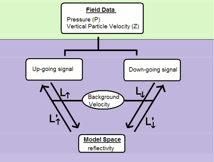
Flowchart
Figure 4. Pressure (P) and vertical particle velocity (Z) data are converted into up- and down-going data. The up- and down-going data are then migrated separately using a modified grid shown in Figure 3. Inversion is performed with residuals in the up/down data domain. |
|
|
In the modified computational grid as shown in Figure 2, the primary signal is obtained by the cross-correlation of the source wavefields with the reflectivity. For the down-going receiver ghost, the receiver nodes are placed at twice the water depth, which effectively represents a reflection off the sea surface.
|
|
|
|
Joint least-squares inversion of up- and down-going signal for ocean bottom data sets |