Geophysical applications of a novel and robust L1 solver

Dix inversion of interval velocity estimation

The Dix equation (Dix, 1952) inverts interval velocities from RMS velocity, which is picked during velocity scanning in prestack seismic data. The equation can be written as

$$v^2_{int(k)} \quad = \quad kV_k^2-(k-1)V_{k-1}^2,$$ (7)

or

$$\sum^k_{i=1}{v^2_{int(k)}} \quad = \quad kV_k^2,$$ (8)

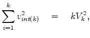where $v$ is interval velocity, $V$ is RMS velocity, and $k$ is the sample number, which can be regarded as travel-time depth. Directly calculating the interval velocity from this formula can easily yield wildly unreasonable results because of the error in the picked RMS velocity. Therefore, it is necessary to solve this problem as a regularized inversion. To linearize the problem, we choose the model space to be the squared interval velocity ($v^2_{int}$ ), instead of the interval velocity itself ($v_{int}$ ).

Thus we can formulate the Dix inversion problem as follows:

$$\boldsymbol{W_d}(\bf {C} \bold u-\bold d) \approx 0,$$ (9)

$$\epsilon \bf {D_{z}} \bold u \approx 0.$$ (10)

In the data-fitting goal (9), u is the unknown model we are inverting for, d is the known data computed from the RMS velocity, C is the causal integration operator and $\bold W_d$ is a data residual weighting function, which is a measure of to our confidence in the RMS velocity. In the model-styling goal (10), $\bold D_{z}$ is the vertical derivative of the velocity model and $\epsilon$ is the weight controlling the strength of the regularization.

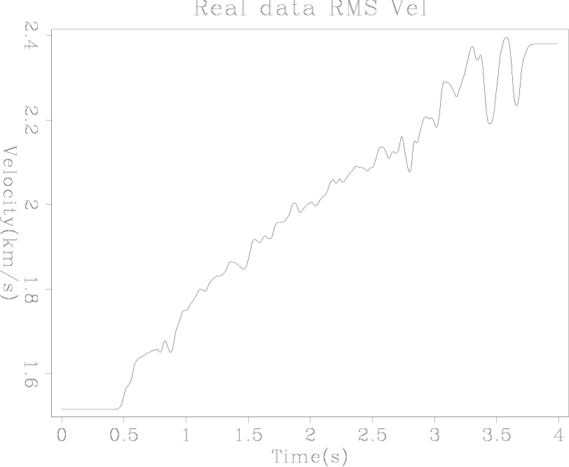
The input RMS velocity with 1000 samples is shown in Figure 1. It is obvious that the violent variation at the end of the trace is not realistic. Thus, we use the hybrid-norm to ignore the large residuals in the data-fitting, which are considered to be noise. At the same time, to obtain a blocky interval velocity model, the large residual in the derivative of the interval velocity should be ``invisible'' to the measure. Therefore, the hybrid norm on the model styling appear to be the best choice.

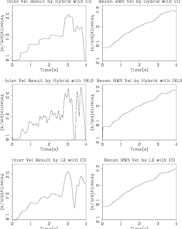
To compare the inversion result, we also use the IRLS and L2 solver on the same data with comparable parameters. The inversion results are shown in Figure 2. The left column is the inverted interval velocity, while the right column is the corresponding reconstructed RMS velocity. The result shows that compared with the IRLS and L2 result, the hybrid solver successfully retrieved the most blocky velocity model, and the corresponding reconstructed RMS velocity contains less noise while keeping the trend of the original data.

input-dix-real Figure 1. Input 1-D RMS velocity.

dix-real
Figure 2. Comparison of the inversion results. Panels in the left column are the estimated interval velocity, while panels on the right are the corresponding reconstructed RMS velocity. Top panels: results of the hybrid with CD; Middle panels: results of the hybrid with IRLS; Bottom panels: results of the L2 norm with CD. Notice that although the reconstructed RMS velocity from the three methods are more or less the same, the interval velocity from hybrid CD is more blocky then the other two.

Geophysical applications of a novel and robust L1 solver