Blocky velocity inversion by hybrid norm

ELF Dataset

In this section, we will estimate an interval velocity model of the North Sea data provided by ELF. There is a known salt body in the middle of this data, which makes it a proper test case for our blockiness goals. Also, this dataset has better spatial sampling than the previous dataset, and can thus better illustrate the differences between the different inversion results. This is also four-second dataset, at a sampling of 5.9 ms. The offset axis has 143 traces starting at 0 m with an increment of 25 m. There are 537 CMP gathers with a spacing of 25 m. Figure 11(b) shows the results of autopicking the dataset, which was constrained by the background RMS velocity, and Figure 11(a) shows the results of direct Dix conversion, as defined above. Figure 12 shows the strength of the picks in the velocity scans.

elf0
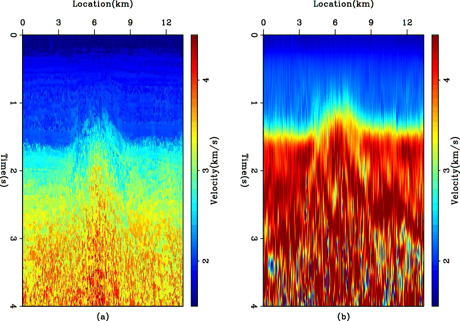
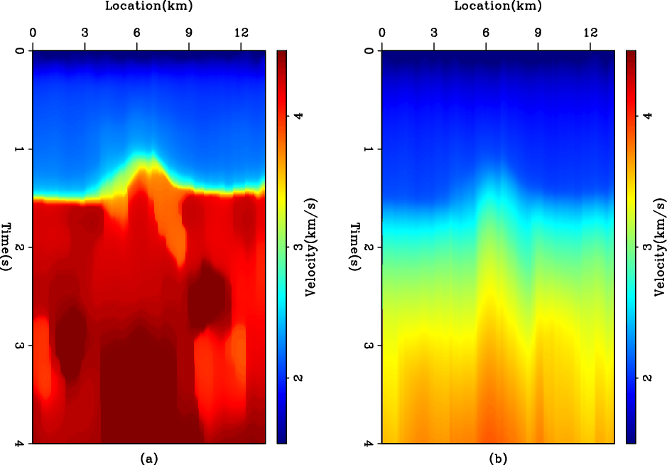
Figure 11. The ELF dataset. (a) The input RMS velocity which is automatically picked from the CMP gathers. (b) The interval velocity by direct Dix conversion.

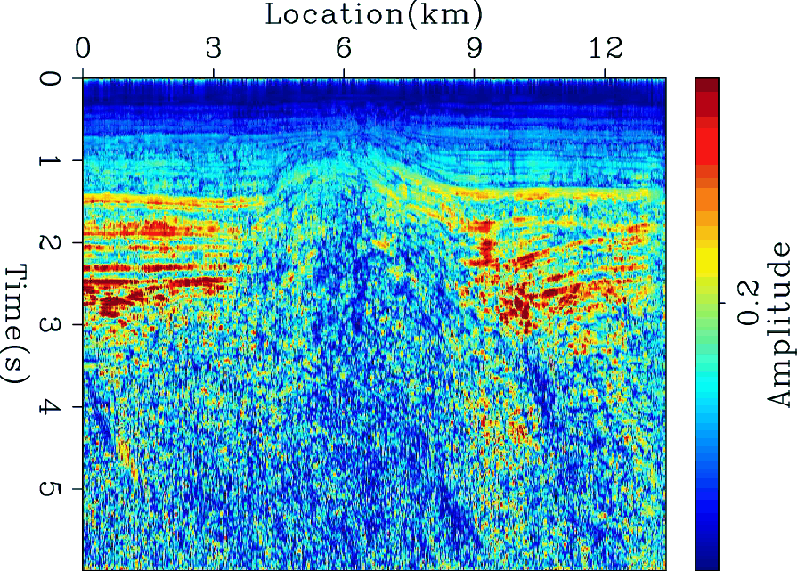
elf-weight Figure 12. The strength of the picks in the velocity scan of ELF dataset, which is used as the weight before dividing by time.

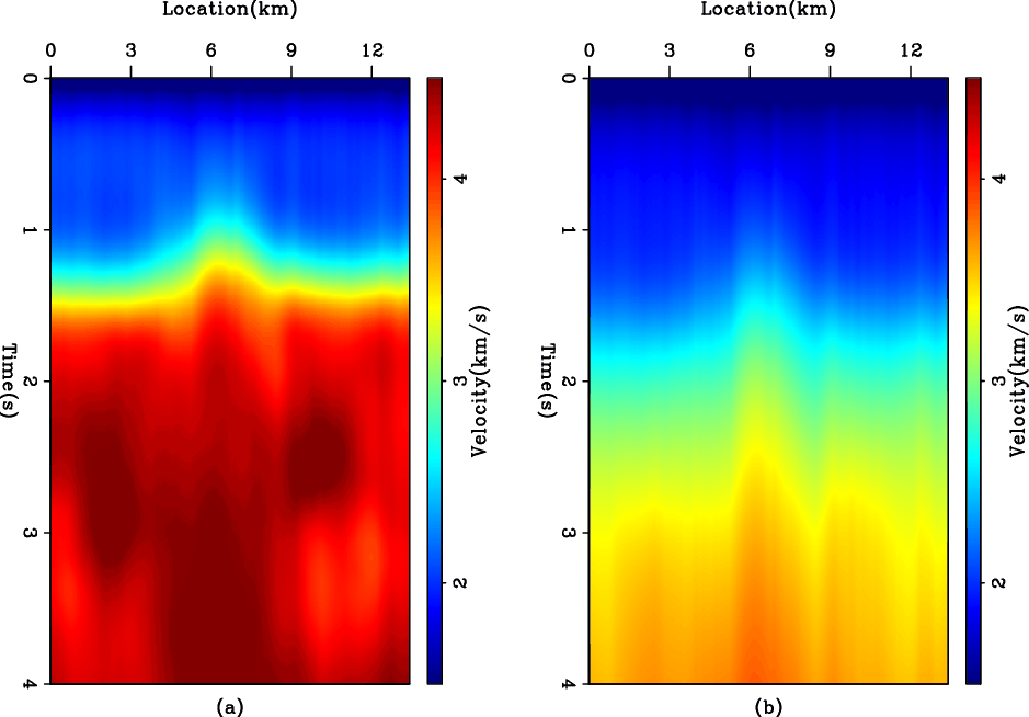
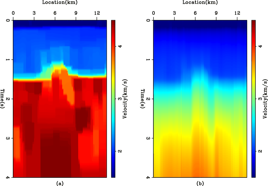
For this dataset, we will only repeat the last two regularizations, which are the first derivative in two and four directions, since they showed the best results with the most symmetric blockiness. Figure 13 shows the results of regularizing in two directions in the $L2$ norm and Figure 14 shows the results of the same regularization in the hybrid norm. Figures 15 and 16 show the results of using four-direction regularization.

Since the dataset is larger with smaller sampling, the improvement of using more directions is evident. Forcing the inversion to pick between two directions has an apparent effect of reducing the resolution. One obvious example is the chalk layer, which looks very horizontal in Figure 14 but more detailed in Figure 16. In all cases, $L2$ always gives smooth results, which smear the model and lower the resolution of the inversion.

l2-elf14
Figure 13. The ELF dataset. (a) The interval velocity estimated by using the first derivative operator in two directions as a regularization in the $L2$ norm. (b) The reconstructed RMS velocity.

hbe-elf17
Figure 14. The ELF dataset. (a) The interval velocity estimated by using the first derivative operator in two directions as a regularization in the hybrid norm. (b) The reconstructed RMS velocity.

l2-elf23
Figure 15. The ELF dataset. (a) The interval velocity estimated by using the first derivative operator in four directions as a regularization in the $L2$ norm. (b) The reconstructed RMS velocity.

hbe-elf29
Figure 16. The ELF dataset. (a) The interval velocity estimated by using the first derivative operator in four directions as a regularization in the hybrid norm. (b) The reconstructed RMS velocity.

Blocky velocity inversion by hybrid norm