|
|
|
|
Dix inversion constrained by L1-norm optimization |
Bube and Langan (1997) and Tang (2006) show that the
nonlinear objective functions, such as the regression equation
(3), can be solved by the IRLS algorithm. Many authors have
demonstrated successful applications of IRLS as a robust estimator to
yield sparse models. To take advantage of the well-established ![]() norm regression, we can transform the problem by introducing a
diagonal weighting function
norm regression, we can transform the problem by introducing a
diagonal weighting function
![]() . Then the fitting goal
2 and the regularization 3 become:
. Then the fitting goal
2 and the regularization 3 become:
| (6) |
One of the most important disadvantages of IRLS algorithm arises in
equation 8: how should we choose the cutoff number
![]() ? We would like to derive this number automatically according
to its physical meaning, instead of cumbersome numerical experiments.
? We would like to derive this number automatically according
to its physical meaning, instead of cumbersome numerical experiments.
Further examining the weighting function, we notice that when applying
the truncated weights, we end up treating small residuals in the ![]() norm, and at the turning point (
norm, and at the turning point (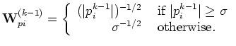 ) we have a sharp transition
to the
) we have a sharp transition
to the ![]() norm. Thus,
norm. Thus, ![]() is the cutoff between the
is the cutoff between the ![]() region
and the
region
and the ![]() region, determining the tolerance to the large
residuals. Therefore, we can choose
region, determining the tolerance to the large
residuals. Therefore, we can choose ![]() according to the desired
blockiness of the model space. For the synthetic example, which is a
40-point-long interval velocity model with three layers, we expect
only two spikes out of those 40 points in the derivative. Therefore we
would like
according to the desired
blockiness of the model space. For the synthetic example, which is a
40-point-long interval velocity model with three layers, we expect
only two spikes out of those 40 points in the derivative. Therefore we
would like ![]() to be around the
to be around the ![]() percentile of the
derivative, allowing 5% of the spikes to be of unlimited size, while
the others are small.
percentile of the
derivative, allowing 5% of the spikes to be of unlimited size, while
the others are small.
|
|
|
|
Dix inversion constrained by L1-norm optimization |