|
|
|
|
Maximum entropy spectral analysis |
Given a discrete (possibly complex) time series
![]() of
of ![]() values with sampling interval
values with sampling interval ![]() (and Nyquist frequency
(and Nyquist frequency
![]() ),
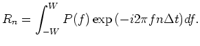
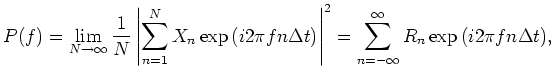
we wish to compute an estimate of the power spectrum
),
we wish to compute an estimate of the power spectrum ![]() , where
, where ![]() is the
frequency. It is well known that
is the
frequency. It is well known that
 is defined by (for
Now suppose that we use the finite sequence
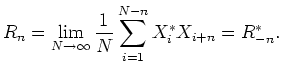 to estimate the first
![]() autocorrelation values
autocorrelation values
![]() . (Methods of obtaining these estimates are
discussed in the section on Computing the Prediction Error Filter.)
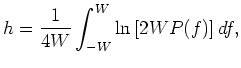
Then, () has shown that maximizing the average entropy
(see Appendix A for a derivation)
. (Methods of obtaining these estimates are
discussed in the section on Computing the Prediction Error Filter.)
Then, () has shown that maximizing the average entropy
(see Appendix A for a derivation)
 for
for
Doing the math, we find that
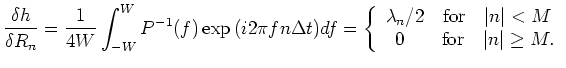 's are Lagrange multipliers to be determined. That the variation of for
's, which are unknown. We can infer from Equation (4)
that
's are Lagrange multipliers to be determined. That the variation of for
's, which are unknown. We can infer from Equation (4)
that
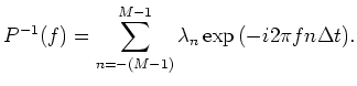 -transform to
:
-transform to
:
 . The first sum in (7) has all of its zeroes outside
the unit circle (minimum phase) and the second sum has its zeroes inside
the unit circle (maximum phase).
. The first sum in (7) has all of its zeroes outside
the unit circle (minimum phase) and the second sum has its zeroes inside
the unit circle (maximum phase).
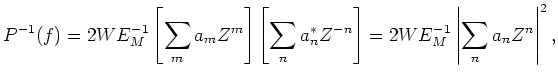
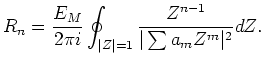
Fourier transforming Equation (1), we find that
is given by the contour (complex) integral
 and at any zero of the maximum phase factor. The poles for .
Equation (10) and its complex conjugate for the
and at any zero of the maximum phase factor. The poles for .
Equation (10) and its complex conjugate for the  are exactly the standard equations for the
maximum and minimum phase spike deconvolution operators
are exactly the standard equations for the
maximum and minimum phase spike deconvolution operators
Notice that, if we define the ![]() matrix
matrix ![]() as the equidiagonal matrix of autocorrelation
values whose elements are given by
as the equidiagonal matrix of autocorrelation
values whose elements are given by
One gap in the analysis should be filled before we proceed. That the variational principle is a
stationary principle (i.e.,
![]() ) is obvious. That it is truly a maximum principle however
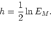
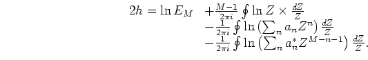
requires some proof. First note that the average entropy
) is obvious. That it is truly a maximum principle however
requires some proof. First note that the average entropy ![]() computed from substituting
(7)
into (3) is exactly
computed from substituting
(7)
into (3) is exactly
 except for ,
and the residue there is
's are the
except for ,
and the residue there is
's are the 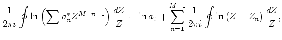 zeroes of the maximum phase factor
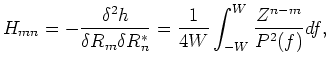
For small deviations from the constraining values of , and from the values of
computed from (8) once ![]() is known, we can expand
is known, we can expand ![]() in a Taylor series:
in a Taylor series:
 's are small deviations in the 's. The
  is an arbitrary complex vector and the equality in
(17) holds only when
is identically zero.
is an arbitrary complex vector and the equality in
(17) holds only when
is identically zero.
The result (17) is sufficient to prove that ![]() is not only stationary, but actually a maximum.
is not only stationary, but actually a maximum.
The analysis given in this section has at least two weak points: (a) For real data, we never measure
the autocorrelation function directly. Rather, a finite time series is obtained and an autocorrelation
estimate is computed. Given the autocorrelation estimate, an estimate of the minimum phase operator must
then be inferred.
A discussion of various estimates of the autocorrelation is given in the next
section on Computing the Prediction Error Filter,
along with a method of estimating the prediction error filter without computing an
autocorrelation estimate. (b) Even assuming we could compute the ``best'' estimate of the autocorrelation,
that estimate is still subject to random error. The probability of error increases as we compute values of
with greater lag ![]() . Since there is a one-to-one correspondence between the 's and the
. Since there is a one-to-one correspondence between the 's and the
![]() 's, the length of the operator can strongly affect the accuracy of the estimated MESA power spectrum.
A method of estimating the optimum operator length for a given sample length
's, the length of the operator can strongly affect the accuracy of the estimated MESA power spectrum.
A method of estimating the optimum operator length for a given sample length ![]() will be discussed
in the subsequent section on Choosing the Operator Length.
will be discussed
in the subsequent section on Choosing the Operator Length.
|
|
|
|
Maximum entropy spectral analysis |