|
 |
 |
 | 3D shot-profile migration in ellipsoidal coordinates |  |
![[pdf]](icons/pdf.png) |
Next: Relationship to elliptically anisotropic
Up: Ellipsoidal Geometry
Previous: Ellipsoidal Geometry
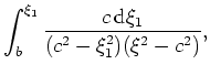
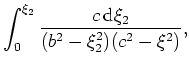
A second definition for confocal ellipsoidal coordinates uses
auxiliary variables defined through integral transforms.
() defines the following Jacobi elliptic integral
transforms for each
coordinate system axis:
where axes
![$ [\beta,\gamma,\alpha]$](img47.png) are conformal to the
are conformal to the
![$ [\xi_1,\xi_2,\xi_3]$](img48.png) axes, but are stretched by the integral
transforms defined in equation 5.
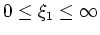
Axes
are defined on the following ranges:
axes, but are stretched by the integral
transforms defined in equation 5.
Axes
are defined on the following ranges:
 ,
,
 and
and
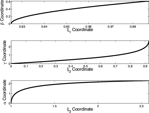
 . Additional information on the integral transforms can be
found in Appendix A. Figure 3 illustrates
the relative stretching for each axis for the wide-azimuth geometry
case presented in figure 2.
. Additional information on the integral transforms can be
found in Appendix A. Figure 3 illustrates
the relative stretching for each axis for the wide-azimuth geometry
case presented in figure 2.
|
|---|
IntegralTransform
Figure 3. Integral transform stretches
for the
 axes given by
equation 5. Top panel: axes given by
equation 5. Top panel:
 coordinate stretch. Middle panel:
 coordinate
stretch. Bottom panel: coordinate
stretch. Bottom panel:
 coordinate stretch.[NR] coordinate stretch.[NR]
|
|---|
![[png]](icons/viewmag.png)
|
|---|
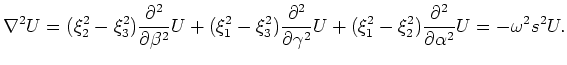
The integral ellipsoidal-coordinate Helmholtz equation is
(, ):
 |
|
|
(A-6) |
Note that this definition effectively rescales the
coordinate axes to eliminate the first-order partial-differential
terms in equation 2. This represents the most
important theoretical result in this paper, as it removes the main
implementation difficulty. In addition, integral ellipsoidal
coordinates are defined globally, not just in octants, which
eliminates the non-uniqueness noted above.
Obtaining a dispersion relationship from the expression in
equation 6 is fairly straightforward. Replacing the
partial differential terms with their Fourier-domain counterparts
(i.e.
 , for
, for
 ) and solving for the
extrapolation direction wavenumber
) and solving for the
extrapolation direction wavenumber  yields
 |
(A-7) |
where
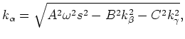 |
(A-8) |
In general, equation 7 is inexact because the 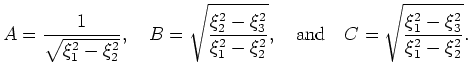 and
and
 coefficients in equations 8 (and possibly slowness)
vary spatially along the
coefficients in equations 8 (and possibly slowness)
vary spatially along the  and
and  axes.
axes.
|
|
|
|
| 3D shot-profile migration in ellipsoidal coordinates | |
|
Next: Relationship to elliptically anisotropic
Up: Ellipsoidal Geometry
Previous: Ellipsoidal Geometry
2009-04-13