3D shot-profile migration in ellipsoidal coordinates

Ellipsoidal Geometry

A common definition of an ellipsoidal coordinate system denoted by $\boldsymbol{\xi}=[\xi_1,\xi_2,\xi_3]$ relative to a Cartesian mesh given by $\boldsymbol{x}=[x_1,x_2,x_3]$ is (, ):

$$x_1^2 = \frac{ (a^2 + \xi_1^2) (a^2+\xi_2^2) (a^2+\xi_3^2) }{(b^2-a^2)(c^2-a^2)},$$

$$x_2^2 = \frac{ (b^2+\xi_1^2) (b^2+\xi_2^2) (b^2+\xi_3^2) }{(a^2-b^2)(c^2-b^2)},$$ (A-1)

$$x_3^2 = \frac{ (c^2+\xi_1^2) (c^2+\xi_2^2)(c^2+ \xi_3^2)}{(a^2-c^2)(b^2-c^2)}.$$

Parameters $a, b,$ and $c$ are constants defining the coordinate system ellipticity and are constrained by three inequalities: $a^2 < \xi_1^2 < b^2$, $b^2 < \xi_2^2 < c^2$, and $c^2 < \xi_3^2 < \infty$. Surfaces of constant $\xi_3$ are confocal ellipsoids and represent the direction of wavefield extrapolation, while those of constant $\xi_1$ and $\xi_2$ form two- and one-sheeted hyperboloids, respectively. We note that because equations 1 are defined by the squares of the variables, each Cartesian point $\boldsymbol{x}$ is represented by eight ellipsoidal points $\boldsymbol {\xi }$, one located in each octant.

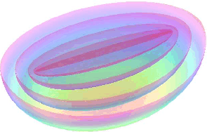
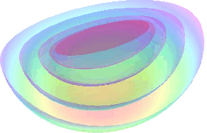
Figures 1 and 2 present two ellipsoidal coordinate examples. In each figure, we infilled the four octants with positive $\xi_3$ arguments to form a coordinate system appropriate for performing 3D wavefield extrapolation. The difference between the two coordinate systems is controlled by parameter $b$, where decreasing $b$ leads to a more spherical mesh. Note that in this coordinate system waves can propagate in all azimuthal directions, and usually at low angles to the extrapolation direction in typical Gulf of Mexico velocity profiles.

NarrowAzimuth Figure 1. Example of an ellipsoidal coordinate system conforming to narrow-azimuth acquisition geometry created with the parameters $[a,b,c]=[0,0.995,1]$. The figure shows five confocal shells. [NR]

WideAzimuth Figure 2. Example of an ellipsoidal coordinate system conforming to wide-azimuth acquisition geometry created with the parameters $[a,b,c]=[0,0.925,1]$. The figure shows five confocal shells.[NR]

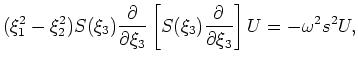
() define the elliptic-coordinate Helmholtz equation as

$$\nabla^2 U = (\xi_3^2-\xi_2^2) S(\xi_1) \frac{\partial}{\partial \xi_1} \left[ S(\xi_1) \frac{\partial}{\partial \xi_1} \right]U +$$

$$(\xi_1^2-\xi_3^2) S(\xi_2) \frac{\partial}{\partial \xi_2} \left[ S(\xi_2) \frac{\partial}{\partial \xi_2} \right] U +$$

$$(\xi_1^2-\xi_2^2) S(\xi_3) \frac{\partial}{\partial \xi_3} \left[ S(\xi_3) \frac{\partial}{\partial \xi_3} \right] U = -\omega^2 s^2 U,$$ (A-2)

where $U$ is a wavefield, $\nabla^2$ is the Laplacian operator, $\omega$ is angular frequency, $s$ is slowness (reciprocal of velocity), and $S(\sigma)$ is a general parameter defined by

$$S(\sigma) = \sqrt{(\sigma^2+a^2)(\sigma^2+b^2)(\sigma^2+c^2)}.$$ (A-3)

Equation 2 contains partial derivatives with respect to the parameter $S$. This leads to a dispersion relationship of the type studied in (),

$$k_{\xi_3} = {\rm i} a_3 \pm \sqrt{ a_4^2 \omega^2 s^2 - a_5^2 k_{... ...^2 - a_6^2k_{\xi_2}^2 + {\rm i}a_8 k_{\xi_1} + {\rm i} a_9 k_{\xi_2}-a_{10}^2},$$ (A-4)

where $a_i$ are geometric coefficients, ${\rm i}=\sqrt{-1}$ and $k_{\xi_j}$ is the wavenumber in the corresponding $j^{th}$ axis.

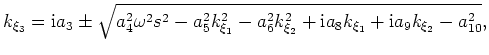
Overall, the ellipsoidal coordinate system as defined in equation 1 is well suited to 3D shot-profile migration in a geometric sense; however, two issues make it difficult to implement accurately. First, the dispersion relationship in equation 4 does not easily lend itself to implicit finite-difference methods because of the imaginary first-order terms (e.g., ${\rm i} a_8 k_{\xi_1}$). Second, the octant-based definition introduces non-uniqueness to the coordinate system variables. Overall, making an ellipsoidal coordinate system practical for wavefield extrapolation will require an alternate definition that overcomes these two issues.

3D shot-profile migration in ellipsoidal coordinates