Angle-domain common-image gathers in generalized coordinates

Polar coordinate example

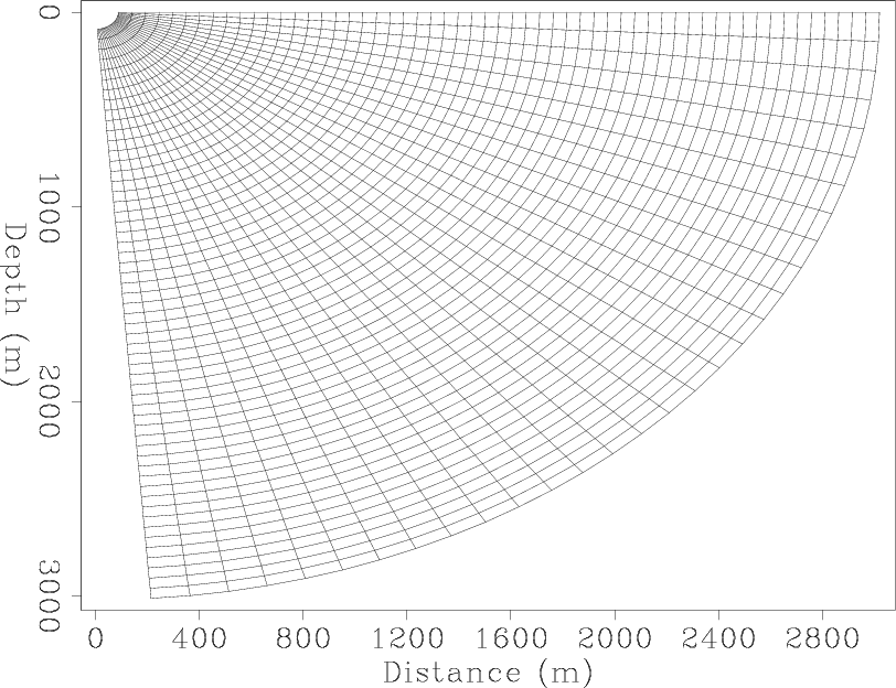
The polar coordinate system, where the extrapolation direction is oriented in the angular rather than the radial direction (see figure 7), is defined by

$$\left[ \begin{array}{c} x_1\\ x_3 \end{array} \right] = \left[ \... ... \, {\rm cos} \,\xi_3 \\ a\,\xi_1\, {\rm sin} \,\xi_3 \\ \end{array} \right].$$ (27)

The partial derivative transformation matrix between the two systems is

$$\left[ \begin{array}{cc} \frac{\partial x_1}{\partial \xi_1}& \fr... ...\ a \, {\rm sin} \, \xi_3 & a \,\xi_1\, {\rm cos} \, \xi_3 \end{array}\right],$$ (28)

leading to the following differential travel-time equations

$$\left[ \begin{array}{c} \frac{\partial t}{\partial h_{\xi_1}}\\ ... ...a \\ a \,\xi_1 \, {\rm cos} \,\xi_3 \, {\rm cos} \,\gamma \end{array} \right].$$ (29)

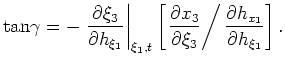
Inserting equations 28 into equation 24 generates the expression for polar coordinate ADCIGs

$${\rm tan}\gamma = \frac{\partial \xi_3}{\partial h_{\xi_1}}\left[\xi_1 \frac{\partial h_{\xi_1}}{\partial {\xi_1}}\right].$$ (30)

Thus, one cannot calculate ADCIGs directly in a polar coordinate system unless the spatial dependency is judiciously eliminated.

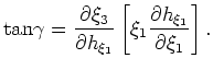The polar coordinate system provides an example where ADCIGs contain a geometric dependence on $\boldsymbol{\xi}$. Inserting the geometric factors $\frac{\partial x_1}{\partial \xi_1}$ and $\frac{\partial x_3}{\partial \xi_3}$ from above into equation 25 leads to

$$\frac{\partial h_{\xi_1}}{\partial {\xi_1}}= \left. \frac{\partia... ...1}{\partial \xi_1}\right/ \frac{\partial x_3}{\partial \xi_3}= \frac{1}{\xi_1}.$$ (31)

Integrating along surfaces of constant $\xi_3$ yields

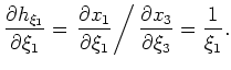$$h_{\xi_1} = {\rm ln} \, \xi_1.$$ (32)

Equation 32 defines the subsurface axis stretch required to directly calculate ADCIGs by Fourier-based approaches.

One question is how best to perform this stretch. One approach would be to perform linear shifting and then regrid that result to an natural log grid. However, the computational overhead renders this method less-than-ideal, especially for situations where estimating $\frac{\partial h_{\xi_1}}{\partial {x_3}}$ directly by slant-stack processing is more efficient. However, this remains an open research topic.

PC Figure 7. Example of a polar coordinate system. [NR]

Angle-domain common-image gathers in generalized coordinates