Next: Specular multiple from dipping
Up: Kinematics of 2D multiples
Previous: General formulation
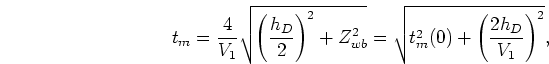
The traveltime of the first-order water-bottom multiple is given by
 |
(15) |
which is simply the traveltime of a primary at twice the depth of the
water-bottom
 .
.
From the symmetry of the problem,
 and
and
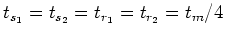 ,
which in turn means
,
which in turn means
 . Furthermore, from
Equations 7 and 8 it immediately follows that
. Furthermore, from
Equations 7 and 8 it immediately follows that
 and
and
 which says that
the traveltimes of the refracted rays are equal to the traveltimes
of the corresponding segments of the multiple. Equation 4 thus simplifies
to
which says that
the traveltimes of the refracted rays are equal to the traveltimes
of the corresponding segments of the multiple. Equation 4 thus simplifies
to
 |
(16) |
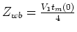
which indicates that the subsurface offset at the image point of a trace
with half surface offset  depends only on the velocity contrast
between the water and the sediments. In particular, if the trace is
migrated with the water velocity, i.e.
depends only on the velocity contrast
between the water and the sediments. In particular, if the trace is
migrated with the water velocity, i.e. 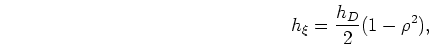 , then
  which proves the property that the multiple is imaged exactly as a primary.
It should also be noted that, since usually sediment velocity is faster than
water velocity, then
which proves the property that the multiple is imaged exactly as a primary.
It should also be noted that, since usually sediment velocity is faster than
water velocity, then  and therefore the multiples are
mapped to subsurface offsets with the opposite sign to
that of the surface offset when migrated with sediment velocity.
and therefore the multiples are
mapped to subsurface offsets with the opposite sign to
that of the surface offset when migrated with sediment velocity.
From Equation 5, the depth of the image point can be easily
computed as
 |
(17) |
which for migration with the water velocity reduces to  ,
showing that the multiple is migrated as a primary at twice
the water depth as is intuitively obvious. Finally, from Equation 6,
the horizontal position of the image point reduces to
,
showing that the multiple is migrated as a primary at twice
the water depth as is intuitively obvious. Finally, from Equation 6,
the horizontal position of the image point reduces to
 |
(18) |
This result shows that the multiple is mapped in the image space
to the same horizontal position as the corresponding CMP even if
migrated with sediment velocity. This result is a direct
consequence of the symmetry of the raypaths of the multiple reflection in this
case. For dipping water bottom or for diffracted multiples this is not the
case (, ).
Equations 16-18 give the image
space coordinates in terms of the data space coordinates. An important
issue is the functional relationship between the subsurface
offset and the image depth, since it determines the moveout of the
multiples in the subsurface-offset-domain common-image-gathers (SODCIGs).
Replacing
 and
and
 in
Equation 17 we get
in
Equation 17 we get
 |
(19) |
which shows that the moveout is a hyperbola (actually, for off-end geometry,
half of a hyperbola, since we already established that 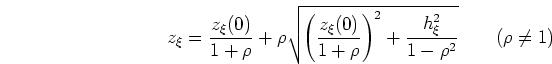 if
if  ).
).
odcig1
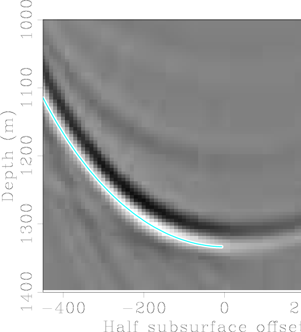
Figure 3. Subsurface offset domain common
image gather of a water-bottom multiple from a flat water-bottom. Water
velocity is 1500 m/s, water depth 500 m, sediment velocity 2500 m/s and
surface offsets from 0 to 2000 m. Overlaid is the residual moveout curve
computed with Equation 19.
|
|
![[pdf]](icons/pdf.png) ![[png]](icons/viewmag.png)
|
|---|
Figure 3 shows
an SODCIG for a specular water-bottom multiple from a flat
water-bottom 500 m deep. The data was migrated with a two-layer
velocity model: the water
layer of 1500 m/s and a sediment layer of velocity 2500 m/s. Larger
subsurface offsets (which according to Equation 16 correspond to
larger surface offsets) map to shallower depths for the usual situation of
 , as we should expect since the rays are refracted to increasingly
larger angles until the critical reflection angle is reached. Also notice that the
hyperbola is shifted down by a factor
, as we should expect since the rays are refracted to increasingly
larger angles until the critical reflection angle is reached. Also notice that the
hyperbola is shifted down by a factor  with respect to
its image point when migrated with water velocity.
with respect to
its image point when migrated with water velocity.
In angle-domain common-image-gathers (ADCIGs), the half-aperture angle
reduces to
 , which in terms of the data
space coordinates is given by
, which in terms of the data
space coordinates is given by
![\begin{displaymath}
\gamma=\sin^{-1}\left[\frac{2\rho h_D}{V_1t_m}\right].
\end{displaymath}](img90.png) |
(20) |
The depth of the image can be easily computed from Equation 14.
In particular, if the data are migrated with the velocity of the water,
then , and therefore
 , which means a horizontal
line in the (
, which means a horizontal
line in the (
 ) plane at twice the depth of the water-bottom.
Equivalently, we can say that the
residual moveout in the (
) plane is zero, once again
corroborating that the water-bottom multiple is migrated as a primary if
.
Equation 14 can be expressed in terms of the data space coordinates
using Equations 16 and 17 and noting that
) plane at twice the depth of the water-bottom.
Equivalently, we can say that the
residual moveout in the (
) plane is zero, once again
corroborating that the water-bottom multiple is migrated as a primary if
.
Equation 14 can be expressed in terms of the data space coordinates
using Equations 16 and 17 and noting that
 |
(21) |
If this expression simplifies to
 ,
which is the aperture angle of a primary at twice the water-bottom depth.
,
which is the aperture angle of a primary at twice the water-bottom depth.
As I did with the SODCIG, it is important to find the functional
relationship between
 and
and  since it dictates the
residual moveout of the multiple in the ADCIG. Plugging
Equations 16 and 17 into equation 14,
using Equations 15, and 20 to eliminate and
simplifying we get
since it dictates the
residual moveout of the multiple in the ADCIG. Plugging
Equations 16 and 17 into equation 14,
using Equations 15, and 20 to eliminate and
simplifying we get
Once again, when the multiple is migrated with the water velocity ()
we get the expected result
 , that is, flat
moveout (no angular dependence). The residual moveout in ADCIGs is therefore
given by
, that is, flat
moveout (no angular dependence). The residual moveout in ADCIGs is therefore
given by
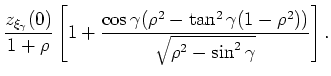
![\begin{displaymath}
\Delta n_{\mbox{RMO}}=z_{\xi_\gamma}(0)-z_{\xi_\gamma}=\left...
...\gamma)}{\sqrt{\rho^2-\sin^2\gamma}}\right]\frac{z_0}{1+\rho}.
\end{displaymath}](img100.png) |
(24) |
This equation reduces to that of Biondi and Symes (2004) when
is small (Appendix C), which is when we can neglect ray bending at the
multiple-generating interface.
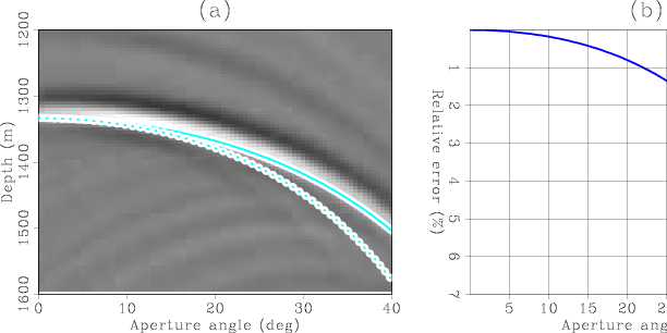
Panel (a) of Figure 4 shows the ADCIG corresponding to the
SODCIG shown in Figure 3. Notice that the migrated depth
at zero aperture angle is the same as that for the zero sub-surface offset in
Figure 3. For larger aperture angles, however, the migrated
depth increases as indicated in equation 23. The continuous line
corresponds to Equation 24 whereas the dotted line corresponds to
the tangent-squared of Biondi and Symes (2004). For this model,
the departure of the straight ray approximation can be more than 5% for large
aperture angles as illustrated in panel (b). The relative error represents
the different between the two approximations divided by that the more accurate
of equation 24.
|
|---|
adcig1
Figure 4. Panel (a) is an ADCIG for a water-bottom multiple
from a two flat-layer model. The dotted curve corresponds to the straight
ray approximation whereas the solid curve corresponds to the ray-bending
approximation. Panel (b) is the relative error between the two approximations.
|
|---|
|
|
|---|
Next: Specular multiple from dipping
Up: Kinematics of 2D multiples
Previous: General formulation
2007-10-24
![$\displaystyle \frac{z_{\xi_\gamma}(0)}{1+\rho}\left[1+\frac{\cos\gamma(\rho^2-\tan^2\gamma(1-\rho^2))}{\sqrt{\rho^2-\sin^2\gamma}}\right].$](img98.png)