Synthetic data example

In this section I introduce a simple 2D synthetic example to illustrate the mapping of a water-bottom and a diffracted multiple from data space to image space. Figure 8 shows the velocity model as well as the raypath of the primaries and multiples that were modeled. Figure 9 shows the zero offset section and the CMP gather at CMP position 2400 m. The depth of the deep reflector was chosen so that the multiples and the deep primary came at about the same zero-offset time and were imaged at about the same depth. Notice that the apex of the moveout curve of the diffracted multiple is not at zero offset. Moreover, the moveout curve is not well represented by a hyperbola. Therefore, we cannot attenuate the diffracted multiple via a standard data-space Radon transform.

synth-vels
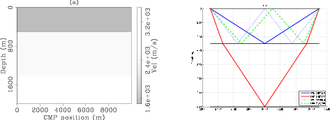
Figure 8. Synthetic model. Panel (a): velocity model. Panel (b): raypaths of modeled primaries and multiples.

synth-cmps
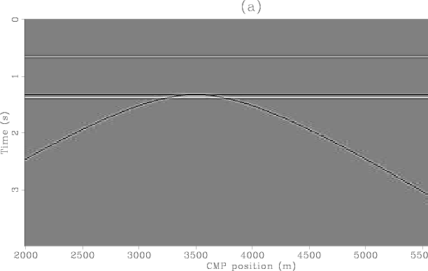
Figure 9. Synthetic data: Panel (a): zero-offset section. Panel (b): CMP gather at CMP location 2400 m.

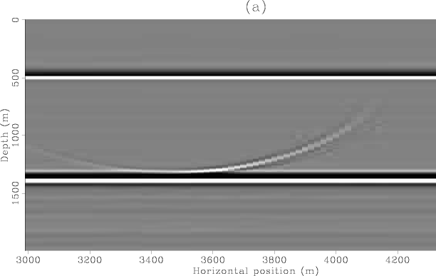
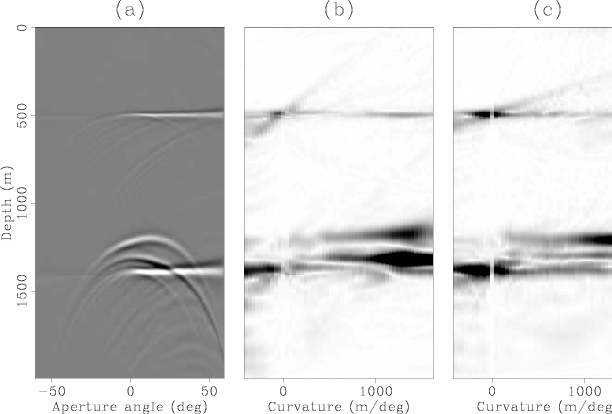
After prestack wave-equation migration, the primaries are well focused at zero subsurface offset as shown in Figure 10. Panel (a) is the zero-subsurface offset section whereas panel (b) is the SODCIG taken at CMP location 3800 m. The water-bottom multiple is mapped to the negative subsurface offsets while the diffracted multiple is mapped to both positive and negative subsurface offsets. Notice that in the zero subsurface offset (panel (a)) the water-bottom multiple and the deep primary are imaged at about the same depth. After transformation to ADCIGs, the primaries are now flat whereas the multiples shows the expected over-migrated residual moveout (panel (a) of Figure 11). The apex of the diffracted multiple, however, is not at zero aperture angle. Panel (b) of Figure 11 shows the Radon plane taken at zero apex shift while panel (c) shows the Radon plane taken at the apex-shift of the multiple (14 degrees). Notice that both the primaries and the water-bottom multiple are well focused in the zero apex-shift plane whereas the diffracted multiple is well focused at its apex-shift plane.

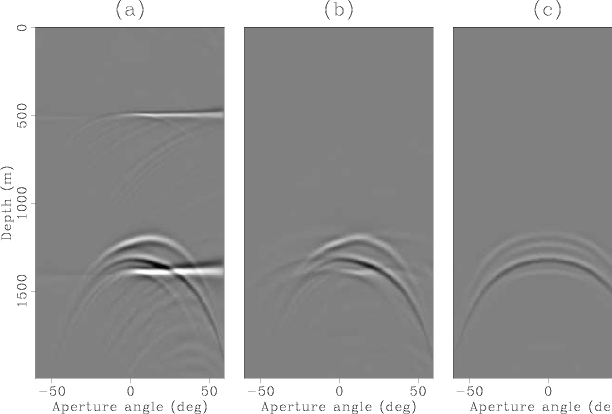
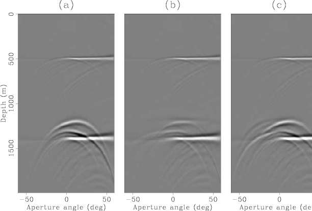
For the sake of comparison, I also applied the non apex-shifted transform to the data and eliminated the primaries with the same mute pattern. After inverse Radon transforming the multiples and subtracting them from the original ADCIG I got the results shown in Figure 12. Panel (a) is the original ADCIG. Panel (b) shows the estimated multiples with the apex-shifted transform and panel (c) shows the multiples estimated with the standard transform. The apex-shifted transform was able to recover the diffracted multiple while the standard transform mistook it for a specular multiple and thus produced the wrong multiple moveout. Notice that some primary energy leaked into the estimate of the multiples in panel (b). Figure 13 shows the estimated primaries. Panel (a) is the original ADCIG, panel (b) is the difference between panels (a) and (b) in Figure 10 and therefore is an estimate of the primaries obtained with the apex-shifted transform. Panel (c) is the corresponding estimate with the standard transform. Some residual multiple energy remains above the deep primary in panel (b) but the primary was recovered. The estimation of the primaries could be improved by adaptively matching the estimated multiples to the multiples in the data (as in SRME), before the subtraction. Finally, panel (c) shows that the poor estimate of the diffracted multiple with the standard transform causes it to leak almost unattenuated into the estimate of the primaries.

mig-cmps
Figure 10. Zero-subsurface offset image (a) and SODCIG at surface location 3800 m (b). Notice the residual moveout of the diffracted multiple being mapped to both positive and negative offsets.

mig-adcig
Figure 11. (a): ADCIG of the same SODCIG in panel (b) of Figure 10; (b): plane taken from the apex-shifted Radon cube at $\Gamma =0$; (c): plane taken from the apex-shifted Radon cube at $\Gamma =10$ degrees.

mig-muls
Figure 12. (a): original ADCIG; (b): estimated multiples with the apex-shifted transform; (c): estimated multiples with the standard transform.

mig-prims
Figure 13. (a): original ADCIG; (b): estimated primaries with the apex-shifted transform; (c): estimated primaries with the standard transform.