


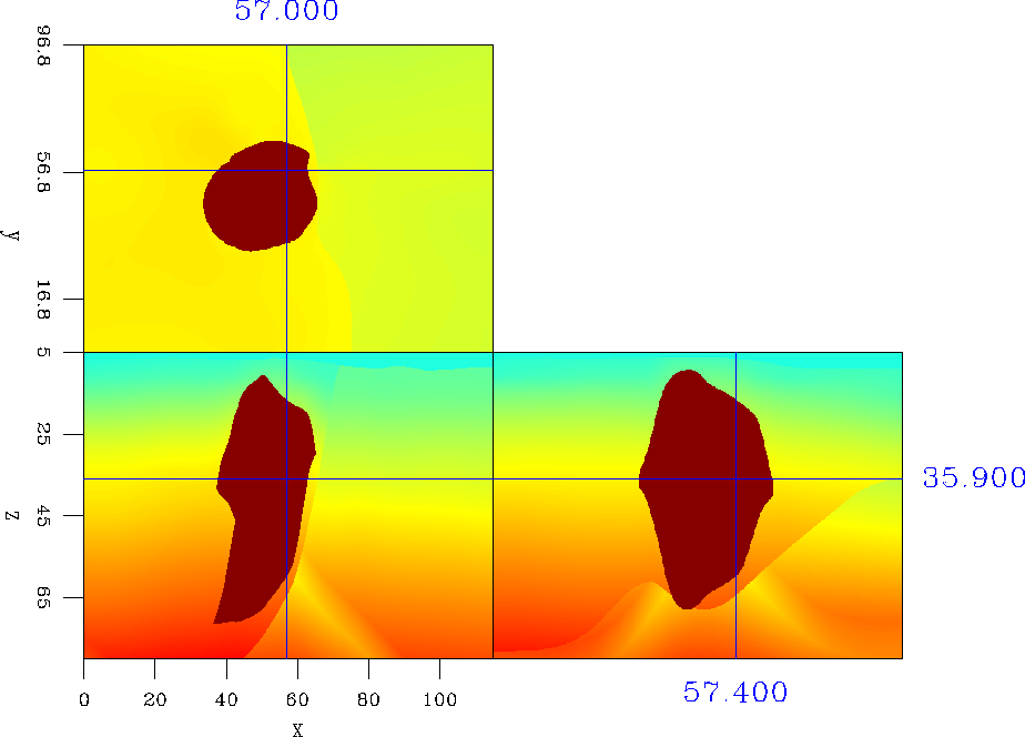
![[*]](http://sepwww.stanford.edu/latex2html/cross_ref_motif.gif) shows the vertical velocity model with a typical salt body.
The salt body is not very complex, but its flank in both the in-line and
cross-line directions are very steep. We obtained the dataset with the velocity and anisotropy parameter models from Exxonmobil.
The vertical velocity and anisotropy parameters were estimated by the integrated velocity model estimation Bear et al. (2005),
which incorporates the surface seismic data with all other data available. For this dataset, in addition to vertical check shots and a substantial
number of sonic logs, there is an offset check shot survey that serve to constrain the estimation of the velocity and anisotropy parameters.
The maximum value of the anisotropy parameters
shows the vertical velocity model with a typical salt body.
The salt body is not very complex, but its flank in both the in-line and
cross-line directions are very steep. We obtained the dataset with the velocity and anisotropy parameter models from Exxonmobil.
The vertical velocity and anisotropy parameters were estimated by the integrated velocity model estimation Bear et al. (2005),
which incorporates the surface seismic data with all other data available. For this dataset, in addition to vertical check shots and a substantial
number of sonic logs, there is an offset check shot survey that serve to constrain the estimation of the velocity and anisotropy parameters.
The maximum value of the anisotropy parameters
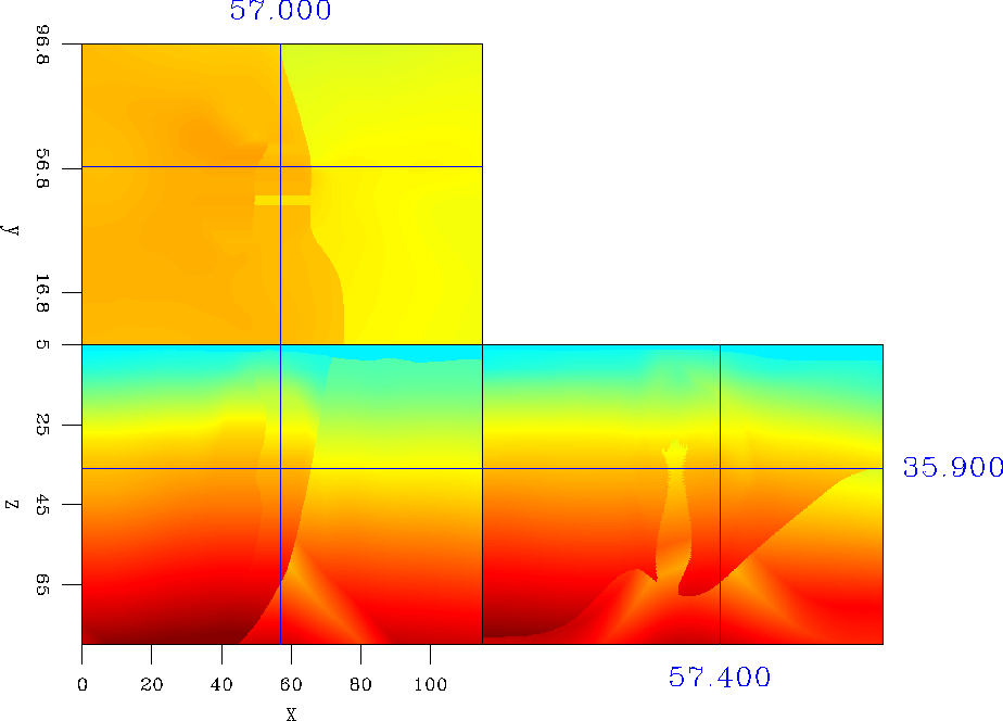
Figure shows the velocity model we used for migration.
We replace the velocity in the salt body with the sediment velocity around it.
We migrate 2700 plane-waves in total. The sampling of ray parameter in both in-line and cross-line directions are 0.000013 s/m. And the maximum take-off angle ![]() is
is
![]() .
The samplings for the cells used for sharing tilted coordinates in Figure are
.
The samplings for the cells used for sharing tilted coordinates in Figure are ![]() and
and ![]() .
.
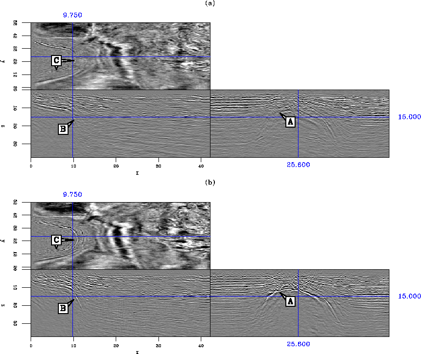
For comparison, we did two migrations: anisotropic plane-wave migration in Cartesian coordinates Shan (2006b) and anisotropic plane-wave migration in tilted coordinates.
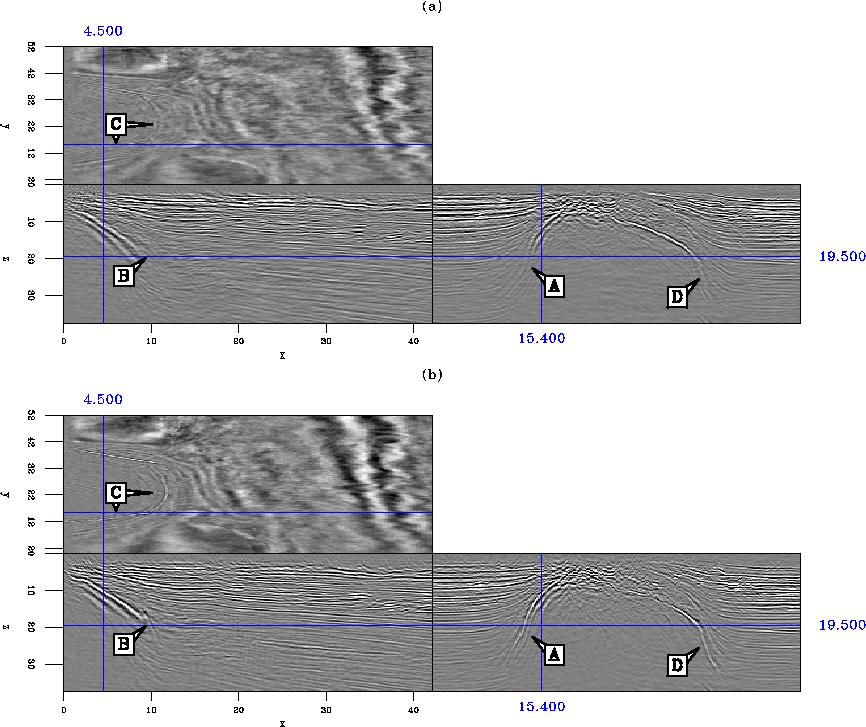
Figures - compare the images of these two migrations at different locations.
In these figures, the top panels are the images obtained by anisotropic plane-wave migration in Cartesian coordinates and
the bottom ones are the images obtained by anisotropic plane-wave migration in tilted coordinates.
In Figure , at "A" in the cross-line section, the top of the salt energy
is dim in Figure (a) while it is strong and continuous in Figure (b).
At "B" in the in-line section, the salt flank is well imaged in Figure (b) while it is absent in
Figure (a).
At "C" in the depth section, we see the continuous salt boundary from the sediment in Figure (b), while we can only see half of it in Figure (a).
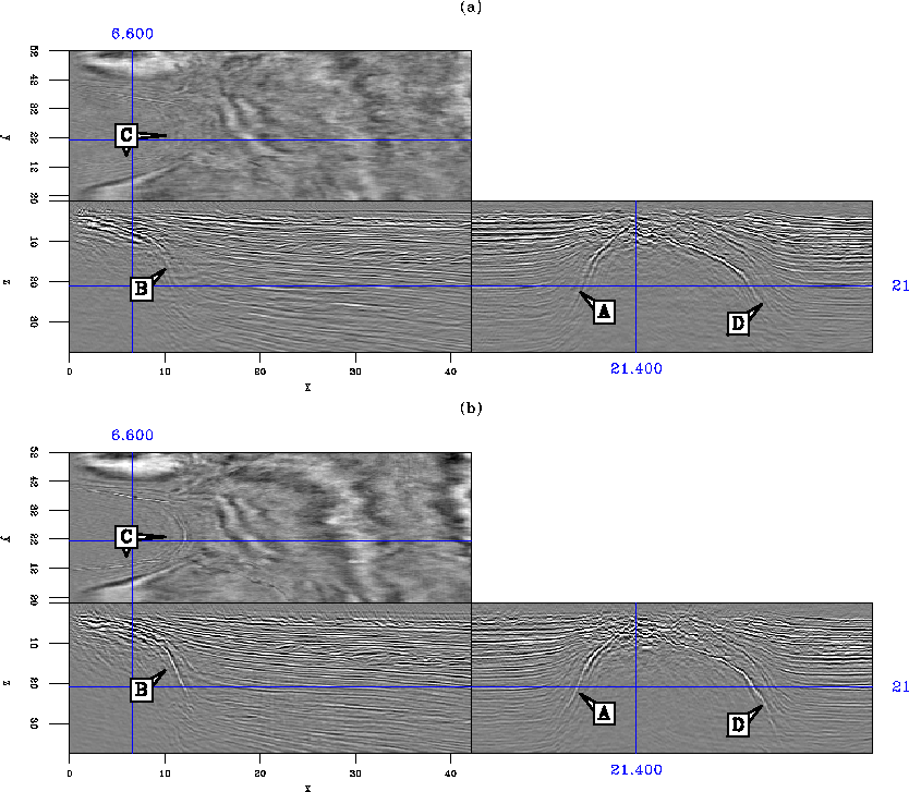
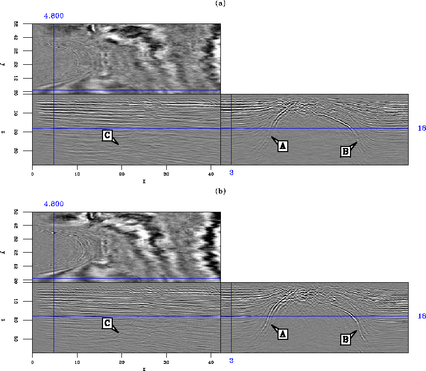
In Figure , at "B" in the in-line section, the salt flank, which is not visible in (a) become
very evident in Figure (b). At "B" in the cross-line section, the salt flank is not imaged at the right
position due to the limit of the accuracy of
the operator in Figure (a) while it is well imaged in Figure (b).
The salt flank at "D" is strong and continuous in Figure (b) but it almost disappears in (a).
At "C" in the depth section, the salt body can be picked out easily from the sediments in (b) but it is not visible in (a).
 |


 |
In Figure , at "B" in the in-line section, the salt flank , which is not visible in Figure (a), is visible in
Figure (b). The top of the salt in the in-line section in Figure (b) is sharper than that in Figure (a).
In the cross-line section of Figure , the plane-wave migration in tilted coordinates images the salt flank at "A" and "D" (Figure (b)), which are very weak and not at the right position in Figure (a). In the depth section, we can see the salt boundary clearly in (b) while they are not visible in Figure (a).
In Figure we can see similar improvements of the salt flanks at "A" and "B".
At "C", we can also see the steeply dipping faults in Figure (b) are much better imaged than that in Figure (a).
From these comparisons, we find that plane-wave migration in tilted coordinates greatly improves the images of the salt body and steeply dipping faults.
 |
 |
 |
 |