Next: Conclusions and Future Work
Up: Curry: Non-stationary interpolation in
Previous: Non-stationary f-x interpolation
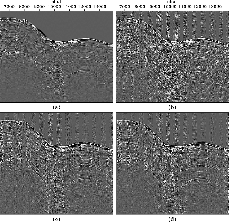
Figure ![[*]](http://sepwww.stanford.edu/latex2html/cross_ref_motif.gif) shows various interpolations of a common-offset section
from a sail line from a 3D marine survey. Figure (a) shows
the original common-offset section, (b) is a 2D interpolation
where the only input to the interpolation is what is shown in Figure (a).
Figure (c) shows the result of a 3D interpolation where a single receiver cable
as well as the common-offset section from the sail line in (a) were used. Figure (d)
is the result of a 4D interpolation, where all four receiver cables were used as well as what was used in (c).
The most obvious issue with all of the interpolations is the introduction of
noise before the water bottom reflection. This is a result of the assumption
of stationarity in time, putting all dips at all times. This noise is much
more prevalent in the 2D interpolation than in the 3D and 4D interpolations.
The quality of the 3D interpolation on the whole is much higher than the 2D
interpolation, whereas the 4D interpolation is almost identical to the 3D case.
This is not overly surprising since there are only 4 points in the 4th dimension
(cross-line offset) which do not contribute much to the result.
shows various interpolations of a common-offset section
from a sail line from a 3D marine survey. Figure (a) shows
the original common-offset section, (b) is a 2D interpolation
where the only input to the interpolation is what is shown in Figure (a).
Figure (c) shows the result of a 3D interpolation where a single receiver cable
as well as the common-offset section from the sail line in (a) were used. Figure (d)
is the result of a 4D interpolation, where all four receiver cables were used as well as what was used in (c).
The most obvious issue with all of the interpolations is the introduction of
noise before the water bottom reflection. This is a result of the assumption
of stationarity in time, putting all dips at all times. This noise is much
more prevalent in the 2D interpolation than in the 3D and 4D interpolations.
The quality of the 3D interpolation on the whole is much higher than the 2D
interpolation, whereas the 4D interpolation is almost identical to the 3D case.
This is not overly surprising since there are only 4 points in the 4th dimension
(cross-line offset) which do not contribute much to the result.
coffsetcomp
Figure 4 Interpolation of a common-offset section.
(a) Input data. (b) 2D interpolation in shot,frequency. (c) 3D interpolation in shot, offsetx, frequency.
(d) 4D interpolation in shot, offsetx, offsety, frequency.


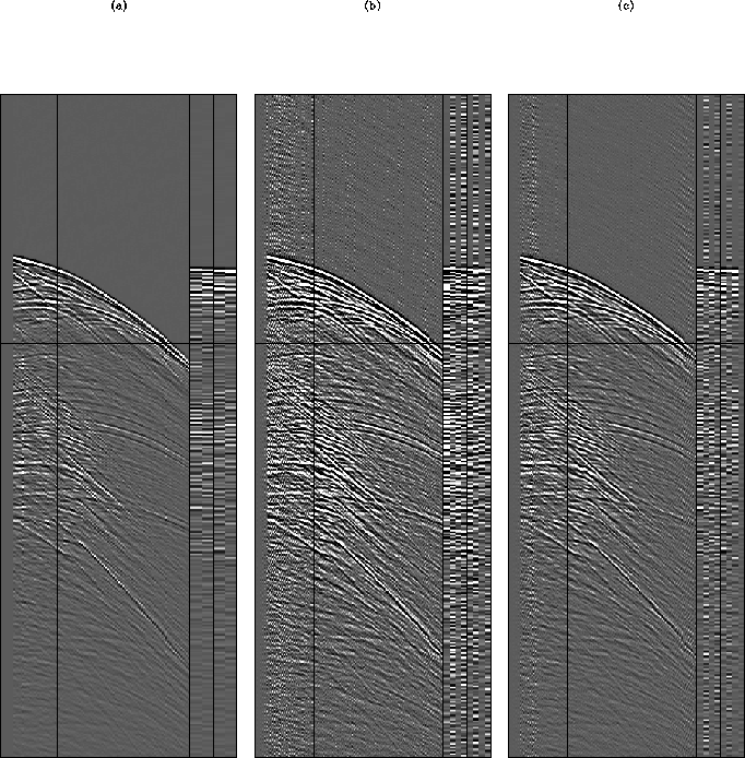
 shotcomp1
Figure 5 Interpolation of a single shot. The front panel is a recorded cable.
(a) Input data with 4 streamers.
(b) 3D interpolation of receivers along a cable.
(c) 4D interpolation in shot, offsetx, offsety, frequency of same shot as in (a).
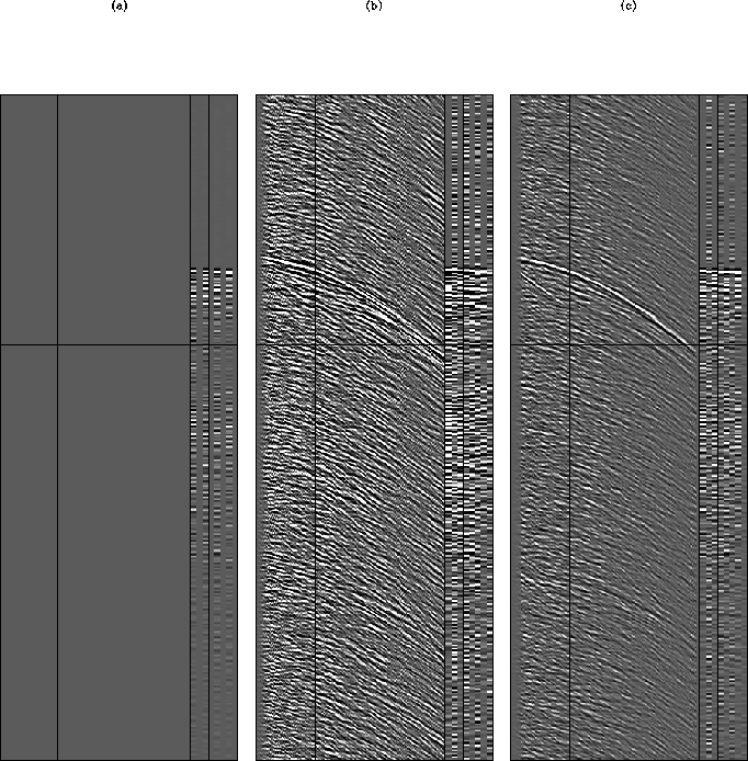
shotcomp2
Figure 6 Interpolation of a single shot. The front panel is an interpolated cable
(a) Input data.
(b) 3D interpolation of a streamer using a single shot.
(c) 4D interpolation in shot, offsetx, and offsety, using multiple shots.
Next, I compare the interpolation of receiver cables using a 3D and a
4D interpolation for a single shot. Figure shows a 3D shot with
the front panel as a recorded receiver cable, interpolated by a factor of 2. The number
of cables is also interpolated from 4 to 8. There is an obvious improvement associated with
moving from a 3D to 4D interpolation. In Figure the same shot is
interpolated in 3D and 4D, but the front panel of the cubes now show an interpolated receiver cable.
This result looks poor in both cases, although noticeably better for the 4D interpolation.
The issue of non-stationarity in time is crippling, although the overall trend of the
water-bottom arrival is captured in both cases. In combination with the previous Figure shows how
the length of the axis being added to the interpolation has a profound effect on the result. The interpolated
cables are of much worse quality than the interpolated inline receivers, which is due to both the larger distance
between the cables and the small number of receiver cables in the acquisition.
Next: Conclusions and Future Work
Up: Curry: Non-stationary interpolation in
Previous: Non-stationary f-x interpolation
Stanford Exploration Project
5/6/2007