Non-stationary f-x interpolation

Since seismic data has dips that vary in space and time, the stationary methodology shown in the previous section cannot be blindly applied to entire data sets. Instead the data are either broken up into regions that are assumed to be stationary or the PEF that is estimated on the data is non-stationary. Non-stationary PEFs estimated in the t-x domain have been used to interpolate data with dips varying in both space and time. Non-stationary PEFs that are estimated in f-x can also be used to interpolate data, but since the dimensionality of the filter is less (with no time/frequency component) and the data are Fourier transformed prior to interpolation, the dip spectrum is assumed to be stationary in time.

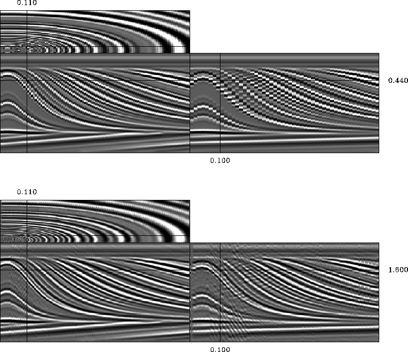
In addition to the issue with time non-stationarity, a time-variable weighting function which could be implemented in t-x could not be implemented in f-x as the frequencies are solved independently. Figure shows the qdome synthetic that is both non-stationary in space and time being interpolated by a factor of 16, 4 in each spatial dimension.

 

nspef
Figure 3 Top: qdome input data; bottom: qdome interpolated by a factor of 4 in each direction. PEF size is 5x5.

The issue of non-stationarity in time in Figure does not appear to be a very large problem. While the flat layers at the top and bottom of the interpolated result do contain some erroneous dips, their amplitude is quite weak compared to the dominant dips in that location.