

Next: Real Data Example
Up: Witten: Optimization
Previous: The Method
A synthetic data example is created to test the algorithm to
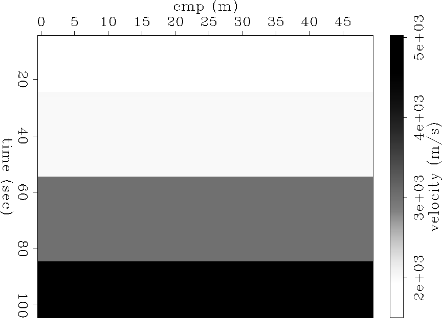
make sure that it works properly. A simple layer-cake earth model is
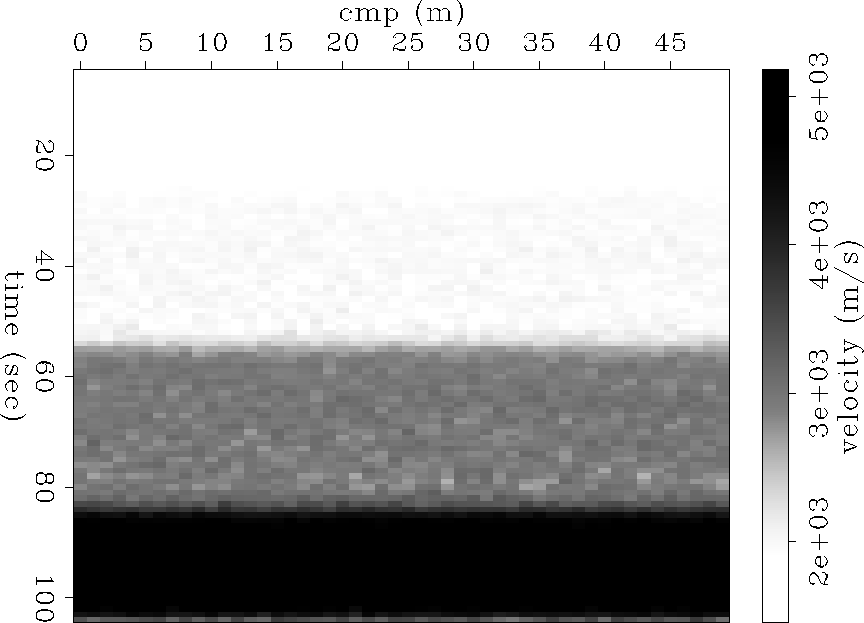
used, shown in Figure ![[*]](http://sepwww.stanford.edu/latex2html/cross_ref_motif.gif) . RMS velocities are then
created from this model as input data to the algorithm. If the
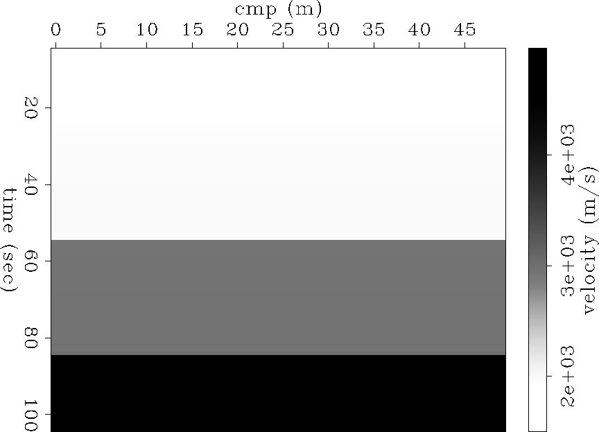
inversion is run on this simple model, the
result is almost perfect, as shown in Figure
. RMS velocities are then
created from this model as input data to the algorithm. If the
inversion is run on this simple model, the
result is almost perfect, as shown in Figure ![[*]](http://sepwww.stanford.edu/latex2html/cross_ref_motif.gif) . The
inversion is off by a maximum of 3%, which occurs at the bottom-most
interface. This error could most likely be reduced further if we
decrease the stopping criterion.
. The
inversion is off by a maximum of 3%, which occurs at the bottom-most
interface. This error could most likely be reduced further if we
decrease the stopping criterion.
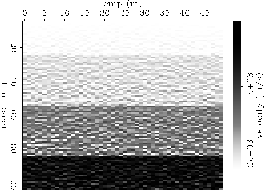
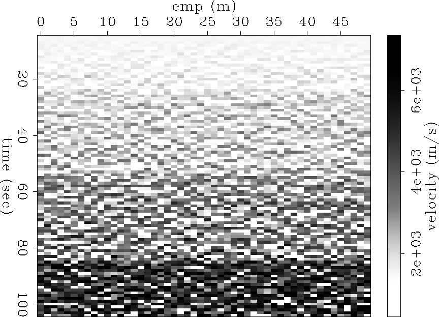
Now 1 and 5 percent Gaussian noise is added to the RMS velocities to simulate real
data. The inversion of this noisy data with very little
smoothness applied is shown in Figures ![[*]](http://sepwww.stanford.edu/latex2html/cross_ref_motif.gif) and
and ![[*]](http://sepwww.stanford.edu/latex2html/cross_ref_motif.gif) . The
noise introduced to the model shows up as block features. As more noise
is added the layers become harder to distinguish from each other.
. The
noise introduced to the model shows up as block features. As more noise
is added the layers become harder to distinguish from each other.
model
Figure 1 A simple layer cake earth model


 Modvint
Figure 2 Inversion result for simple model using the algorithm above. For the simple model shown in Figure
![[*]](http://sepwww.stanford.edu/latex2html/cross_ref_motif.gif) , the result is almost perfect.
, the result is almost perfect.


 ModvintNoise
Figure 3 Inversion of the data with 1% noise.
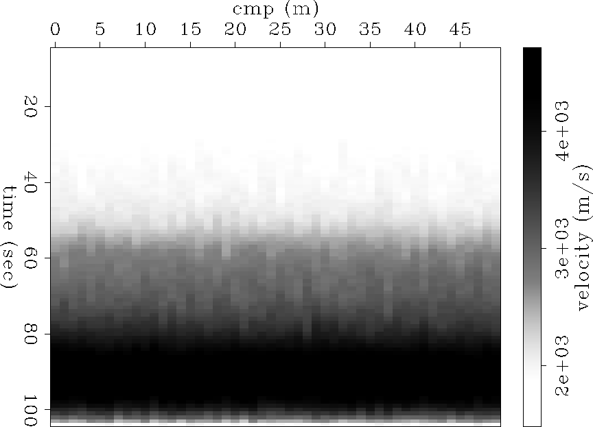
The layer boundaries are still visible, but the noise pollutes the results substantially.


 ModvintNoise5
Figure 4 Inversion of noisy data with 5% noise. The noise is severe enough that the boundary layers are no longer discernible.


If we increase the smoothing parameters on the  regularization, then much of the noise is smoothed out in the result
(Figure
 ![[*]](http://sepwww.stanford.edu/latex2html/cross_ref_motif.gif) and Figure
and Figure
![[*]](http://sepwww.stanford.edu/latex2html/cross_ref_motif.gif) ). If the regularization parameters,
). If the regularization parameters,
 are increased further then the result will be even smoother (Figure
![[*]](http://sepwww.stanford.edu/latex2html/cross_ref_motif.gif) and Figure
and Figure
![[*]](http://sepwww.stanford.edu/latex2html/cross_ref_motif.gif) ).
).
As seen in these examples, it is important to correctly choose the
regularization parameter to get a good inversion result that is
compromise between desired blockiness and introducing spurious
elements into the model in the form high spatial frequency events.
ModvintNoiseSmooth
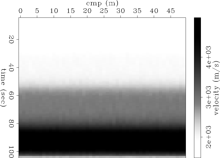
Figure 5 Smoothed version the data with
1% noise. Much of the noise has been smoothed out, but the sharp
boundary contacts are still clear.


 ModvintNoiseSmooth5
Figure 6 Smoothed version of the
data with 5% noise. The smoothing parameter had to be increased to
get rid of much of the noise. The boundaries are more evident here
than in Figure ![[*]](http://sepwww.stanford.edu/latex2html/cross_ref_motif.gif) , but the layer
boundaries are smoothed out.
, but the layer
boundaries are smoothed out.


It can be seen that not all the noise is smoothed out in either Figure
![[*]](http://sepwww.stanford.edu/latex2html/cross_ref_motif.gif) or Figure
or Figure ![[*]](http://sepwww.stanford.edu/latex2html/cross_ref_motif.gif) . This
is because if boundaries are sharp then the
. This
is because if boundaries are sharp then the  regularization preserves them. The sharper the boundary, the higher the
 needs to be smooth them
out. Much of the sharp contrast, however, is also smoothed away. From
this test it became clear the smoothing along the midpoint is not currently
working properly.
ModvintNoiseSmooth2
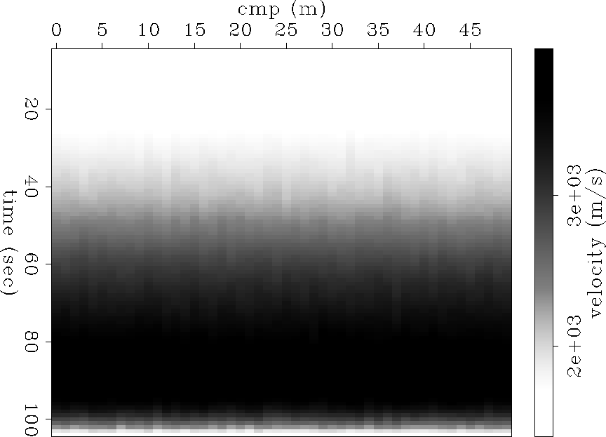
Figure 7 The smoothing parameters were increased
further for the 1% noise. Most of the noise is no longer visible,
but the layer boundaries are not as sharp.


 ModvintNoiseSmooth2-5
Figure 8 Smoothing parameters were
increased for the 5% noise to the point that almost no noise is
visible. Doing this, however, has smoothed out the entire result.


Next: Real Data Example
Up: Witten: Optimization
Previous: The Method
Stanford Exploration Project
5/6/2007
![[*]](http://sepwww.stanford.edu/latex2html/cross_ref_motif.gif) . RMS velocities are then
created from this model as input data to the algorithm. If the
inversion is run on this simple model, the
result is almost perfect, as shown in Figure
. RMS velocities are then
created from this model as input data to the algorithm. If the
inversion is run on this simple model, the
result is almost perfect, as shown in Figure ![[*]](http://sepwww.stanford.edu/latex2html/cross_ref_motif.gif) . The
inversion is off by a maximum of 3%, which occurs at the bottom-most
interface. This error could most likely be reduced further if we
decrease the stopping criterion.
. The
inversion is off by a maximum of 3%, which occurs at the bottom-most
interface. This error could most likely be reduced further if we
decrease the stopping criterion.
