Trade-off between the different parameters - the right-hand singular vectors

To analyze the trade-off between the different anisotropic parameters, we study the null space of the matrix $\mathbf{F}$, i.e. its right-hand vectors associated with the smallest (or zero) singular values. By definition, a right-hand singular vector $\mathbf{v}$ of the matrix $\mathbf{F}$ is such that $\mathbf{F}\mathbf{m}=\mathbf{0}$;as such, if $\mathbf{v_0}$ is solution of $\mathbf{F}\mathbf{v_0}=\mathbf{d}$ and $\mathbf{v}$ is a right-hand singular vector of the matrix $\mathbf{F}$, then any vector $\mathbf{v_0}+\lambda \mathbf{v}$, $\lambda \in \Re$ is also a solution. Consequently, the subspace of the right-hand singular vectors is unconstrained by the equation $\mathbf{F}\mathbf{v}=\mathbf{d}$ and can take any value.

The top panel of figure 3 illustrates the right-hand singular vector (two components) associated with the smallest singular value of $\mathbf{F}$ as the aperture-angle range changes. The condition number is illustrated in the lower panel. Note that when the aperture-angle range is small, the main component of the right-hand singular vector associated with the smallest singular value is V_H. Thus, when the aperture angle range is small, the horizontal velocity cannot be accurately determined because of insufficient data. This confirms our observation why the condition number takes large values with small aperture data.

Eventually, when the aperture-angle range is around $45^{\circ}$, the two components of the right-hand hand singular vector associated with the smallest eigenvalue are of the same order of magnitude. This shows that there is a slight trade-off between the two anisotropic parameters. It is consistent with the fact that the condition number is low and that the problem is well-posed for that range of aperture angles.

 

Sing_vectors Figure 3 Top panel: Right-hand side singular vector (two components) associated with the smallest singular value of 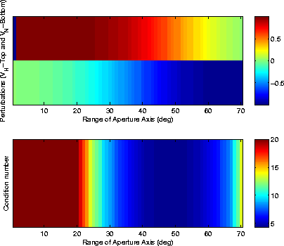${\bf F}$ as a function of the aperture angle range. Bottom panel: Condition number as a funciton of the aperture angle range

We can draw several conclusions from this theoretical study of the estimation problem as an ^M inverse problem.

First, assuming data are noise-free, the sampling interval of the aperture-angle axis has no impact on the estimation of the anisotropic parameters. When taking into account noise in the data, the smaller the sampling interval, the more robust the estimation of the anisotropic parameters.

Second, depending on the data available, different estimation techniques should be used. When only small-aperture data is available, V_H cannot be accurately resolved. As a consequence, it is important to put some additional constraints on V_H so that it does not take extreme values. When large-aperture data is available, V_N and V_H can both be estimated. However, the preceding section showed that trying to estimate both parameters using a usual inversion scheme leads to poor estimates. Two approaches can be used to solve that problem: the first would be to estimate the two anisotropic parameters independently and successively; the second would be to modify the cost function, using weighted least-squares for example. As we seldom have seismic data with aperture range larger than $45^{\circ}$ in the target of interest, the latter approach has to be preferred.

The following table illustrates the results of the updating process for the three different synthetic cases presented above. It shows that although the velocity spectra seemed to give inaccurate results, the estimation process actually improves the overall estimation of the anisotropic parameters.

$$\rho \tilde{\rho} \hat{\rho}$$

$$\left(0.99,0.99,0.99\right) \left(1.005,0.985,0.995\right) \left(0.985,1.005,0.995\right)$$ 1% Perturbation

$$\left(0.90,0.90,0.90\right) \left(0.96,0.80,0.93\right) \left(0.9375,1.125,0.968\right)$$ 10% Perturbation

$$\left(1.00,0.8197,1.075\right) \left(1.05,0.80,1.062\right) \left(0.95,1.025,1.012\right)$$ Isotropic pertubation