


Next: Conclusions
Up: Lomask: Improved flattening with
Previous: Constrained solution with weights
I conducted tests of this constrained flattening method on
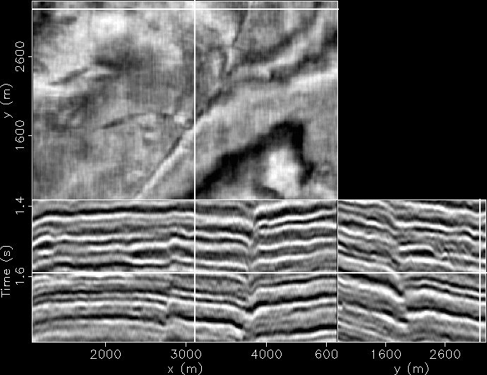
a 3D data set from the Gulf of Mexico. This example illustrates how a single pair of traces can be manually correlated and passed to the constrained flattening method to reconstruct across faults.
shoal_flt
Figure 1 Gulf of Mexico data. The black lines superimposed onto the orthogonal sections identify the location of these sections: a time slice at time= , an in-line section at y=
 , and a cross-line section at x=
 . The reference trace is located at x=
 and y=
 .
.
shoal_flt_wt
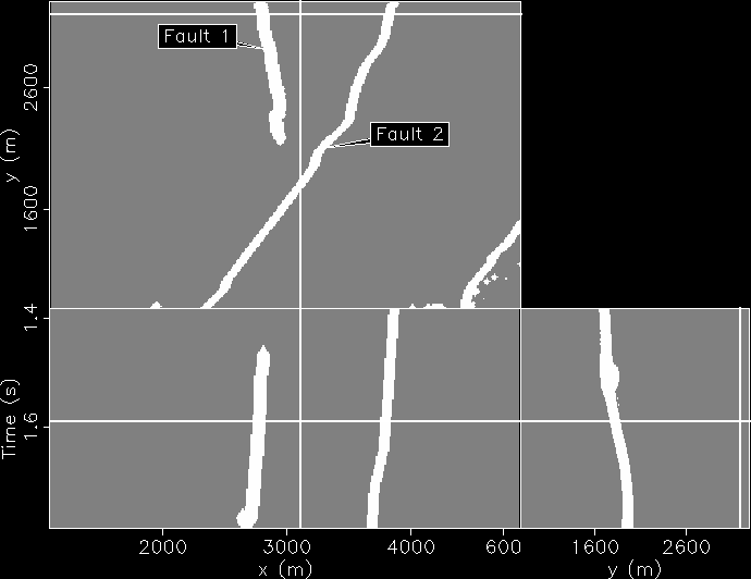
Figure 2 As Figure ![[*]](http://sepwww.stanford.edu/latex2html/cross_ref_motif.gif) displaying the manually picked fault model used for flattening.
displaying the manually picked fault model used for flattening.
shoal_flt_flat
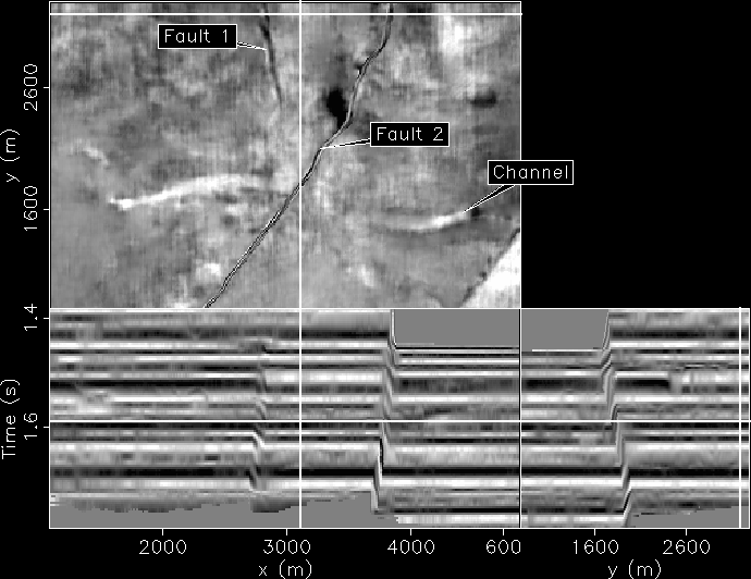
Figure 3 As Figure ![[*]](http://sepwww.stanford.edu/latex2html/cross_ref_motif.gif) only after flattening. Notice that reflectors on both sides of both faults are properly reconstructed. Also, notice a sinusoidal channel that is annotated on the horizon slice.
only after flattening. Notice that reflectors on both sides of both faults are properly reconstructed. Also, notice a sinusoidal channel that is annotated on the horizon slice.
shoal_flt_flat2
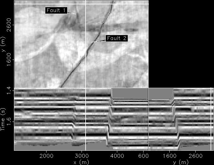
Figure 4 As Figure ![[*]](http://sepwww.stanford.edu/latex2html/cross_ref_motif.gif) except displaying a different horizon slice, time=
except displaying a different horizon slice, time= . Several stratigraphic channel features are visible.
shoal_flt_tau
Figure 5 As Figure ![[*]](http://sepwww.stanford.edu/latex2html/cross_ref_motif.gif) showing the
showing the  field used for flattening.
shoal_flt_pck
Figure 6 As Figure ![[*]](http://sepwww.stanford.edu/latex2html/cross_ref_motif.gif) only displaying every 25th tracked horizon of the Gauss-Newton constrained flattening method. The fault model (solid black) was manually picked.
only displaying every 25th tracked horizon of the Gauss-Newton constrained flattening method. The fault model (solid black) was manually picked.
In Figure ![[*]](http://sepwww.stanford.edu/latex2html/cross_ref_motif.gif) is a 3D Gulf of Mexico data set provided by Chevron. The manually interpreted fault model is displayed in Figure
is a 3D Gulf of Mexico data set provided by Chevron. The manually interpreted fault model is displayed in Figure ![[*]](http://sepwww.stanford.edu/latex2html/cross_ref_motif.gif) . Two faults are identified in the figure. Fault 1 has part of its tip-line encased within the cube as can be observed by its termination in the time slice. Fault 2, on the other hand, does not terminate within the data cube. Because Fault 1 terminates within the data cube, no constraints need to be provided to flatten across it, however, Fault 2 requires some picking. In this case, I picked one vertical pair of traces across Fault 2. Then I applied the weighted Gauss-Newton method with the weight
. Two faults are identified in the figure. Fault 1 has part of its tip-line encased within the cube as can be observed by its termination in the time slice. Fault 2, on the other hand, does not terminate within the data cube. Because Fault 1 terminates within the data cube, no constraints need to be provided to flatten across it, however, Fault 2 requires some picking. In this case, I picked one vertical pair of traces across Fault 2. Then I applied the weighted Gauss-Newton method with the weight  being the picked fault model. The binary mask
  is ones for unconstrained model locations and zeros for constrained model locations. The initial model
  is the picked pair of traces correlating across Fault 2.
Figure ![[*]](http://sepwww.stanford.edu/latex2html/cross_ref_motif.gif) is flattened volume of the data in Figure
is flattened volume of the data in Figure ![[*]](http://sepwww.stanford.edu/latex2html/cross_ref_motif.gif) . Notice the horizons are reconstructed across both faults. Notice the faint outline of a channel that is annotated on the figure. Another view of the same cube is displayed in Figure
. Notice the horizons are reconstructed across both faults. Notice the faint outline of a channel that is annotated on the figure. Another view of the same cube is displayed in Figure ![[*]](http://sepwww.stanford.edu/latex2html/cross_ref_motif.gif) . Several stratigraphic features are reconstructed across both faults. In addition to a fault model, the only picks required were from a single trace of correlations across Fault 2. Also, the
. Several stratigraphic features are reconstructed across both faults. In addition to a fault model, the only picks required were from a single trace of correlations across Fault 2. Also, the  field used to flatten this data is displayed in Figure
 ![[*]](http://sepwww.stanford.edu/latex2html/cross_ref_motif.gif) .
.
In Figure ![[*]](http://sepwww.stanford.edu/latex2html/cross_ref_motif.gif) every 25th tracked horizon of the Gauss-Newton constrained flattening method in displayed. Notice the overlain horizons track their respective events across both faults.
In short, I reconstructed this 3D volume by correlating a single pair of traces across a fault. It should be pointed out that an automatic fault indicator could substitute for the fault model, reducing the amount of manual interpretation even further.
every 25th tracked horizon of the Gauss-Newton constrained flattening method in displayed. Notice the overlain horizons track their respective events across both faults.
In short, I reconstructed this 3D volume by correlating a single pair of traces across a fault. It should be pointed out that an automatic fault indicator could substitute for the fault model, reducing the amount of manual interpretation even further.


Next: Conclusions
Up: Lomask: Improved flattening with
Previous: Constrained solution with weights
Stanford Exploration Project
1/16/2007

![[*]](http://sepwww.stanford.edu/latex2html/cross_ref_motif.gif) displaying the manually picked fault model used for flattening.
displaying the manually picked fault model used for flattening.
![[*]](http://sepwww.stanford.edu/latex2html/cross_ref_motif.gif) only after flattening. Notice that reflectors on both sides of both faults are properly reconstructed. Also, notice a sinusoidal channel that is annotated on the horizon slice.
only after flattening. Notice that reflectors on both sides of both faults are properly reconstructed. Also, notice a sinusoidal channel that is annotated on the horizon slice.
![[*]](http://sepwww.stanford.edu/latex2html/cross_ref_motif.gif) except displaying a different horizon slice, time=
except displaying a different horizon slice, time=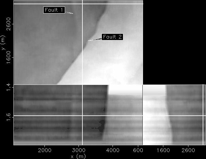
![[*]](http://sepwww.stanford.edu/latex2html/cross_ref_motif.gif) showing the
showing the 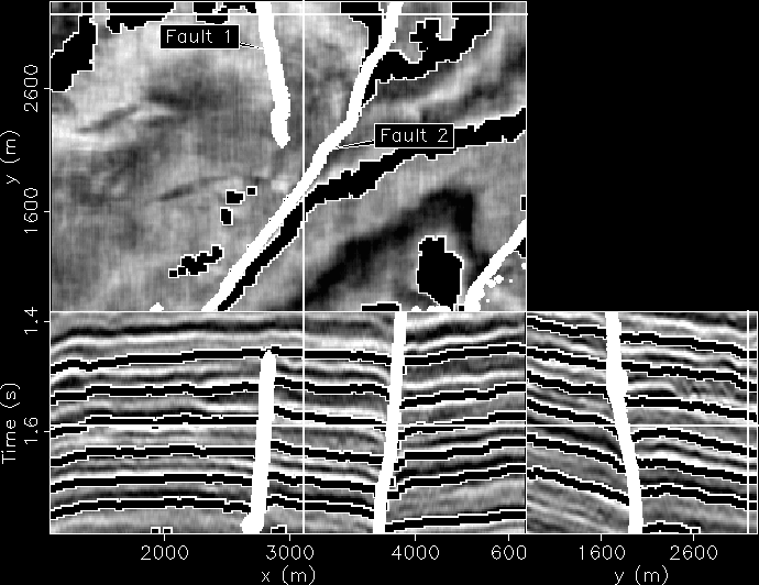
![[*]](http://sepwww.stanford.edu/latex2html/cross_ref_motif.gif) only displaying every 25th tracked horizon of the Gauss-Newton constrained flattening method. The fault model (solid black) was manually picked.
only displaying every 25th tracked horizon of the Gauss-Newton constrained flattening method. The fault model (solid black) was manually picked.
![[*]](http://sepwww.stanford.edu/latex2html/cross_ref_motif.gif) is a 3D Gulf of Mexico data set provided by Chevron. The manually interpreted fault model is displayed in Figure
is a 3D Gulf of Mexico data set provided by Chevron. The manually interpreted fault model is displayed in Figure ![[*]](http://sepwww.stanford.edu/latex2html/cross_ref_motif.gif) . Two faults are identified in the figure. Fault 1 has part of its tip-line encased within the cube as can be observed by its termination in the time slice. Fault 2, on the other hand, does not terminate within the data cube. Because Fault 1 terminates within the data cube, no constraints need to be provided to flatten across it, however, Fault 2 requires some picking. In this case, I picked one vertical pair of traces across Fault 2. Then I applied the weighted Gauss-Newton method with the weight
. Two faults are identified in the figure. Fault 1 has part of its tip-line encased within the cube as can be observed by its termination in the time slice. Fault 2, on the other hand, does not terminate within the data cube. Because Fault 1 terminates within the data cube, no constraints need to be provided to flatten across it, however, Fault 2 requires some picking. In this case, I picked one vertical pair of traces across Fault 2. Then I applied the weighted Gauss-Newton method with the weight ![]() being the picked fault model. The binary mask
being the picked fault model. The binary mask ![]() is ones for unconstrained model locations and zeros for constrained model locations. The initial model
is ones for unconstrained model locations and zeros for constrained model locations. The initial model ![]() is the picked pair of traces correlating across Fault 2.
is the picked pair of traces correlating across Fault 2.
![[*]](http://sepwww.stanford.edu/latex2html/cross_ref_motif.gif) is flattened volume of the data in Figure
is flattened volume of the data in Figure ![[*]](http://sepwww.stanford.edu/latex2html/cross_ref_motif.gif) . Notice the horizons are reconstructed across both faults. Notice the faint outline of a channel that is annotated on the figure. Another view of the same cube is displayed in Figure
. Notice the horizons are reconstructed across both faults. Notice the faint outline of a channel that is annotated on the figure. Another view of the same cube is displayed in Figure ![[*]](http://sepwww.stanford.edu/latex2html/cross_ref_motif.gif) . Several stratigraphic features are reconstructed across both faults. In addition to a fault model, the only picks required were from a single trace of correlations across Fault 2. Also, the
. Several stratigraphic features are reconstructed across both faults. In addition to a fault model, the only picks required were from a single trace of correlations across Fault 2. Also, the ![]() field used to flatten this data is displayed in Figure
field used to flatten this data is displayed in Figure ![[*]](http://sepwww.stanford.edu/latex2html/cross_ref_motif.gif) .
.
![[*]](http://sepwww.stanford.edu/latex2html/cross_ref_motif.gif) every 25th tracked horizon of the Gauss-Newton constrained flattening method in displayed. Notice the overlain horizons track their respective events across both faults.
In short, I reconstructed this 3D volume by correlating a single pair of traces across a fault. It should be pointed out that an automatic fault indicator could substitute for the fault model, reducing the amount of manual interpretation even further.
every 25th tracked horizon of the Gauss-Newton constrained flattening method in displayed. Notice the overlain horizons track their respective events across both faults.
In short, I reconstructed this 3D volume by correlating a single pair of traces across a fault. It should be pointed out that an automatic fault indicator could substitute for the fault model, reducing the amount of manual interpretation even further.