Dipole Coordinates

One simplifying factor for an RWE approach is using a coordinate system that is (nearly) orthogonal, such as that developed from a potential field distribution Shragge (2006b). Accordingly, the coordinate system used in the following investigations is a (nearly) orthogonal mesh derived from the electrostatics potential field distribution, $\Phi$, of a dipole source formed by two static charges  

$$\Phi({\bf x}) = \frac{1}{ \sqrt{ (x-x_1)^2+\xi^2(z-z_1)^2}} - \frac{1}{\sqrt{ (x-x_2)^2+\xi^2 (z-z_2)^2}},$$ (14)

where ${\bf x_1} =[x_1, z_1]$ and ${\bf x_2} =[x_2, z_2]$ are the locations of the two unitary-valued static charges, and $\xi$ is an ellipticity factor inducing a vertical stretch.

A dipolar coordinate system can be derived from equation 14 by computing the equipotential surfaces and associated field lines. Figure 3 illustrates this for a dipole of 4 km spacing and a $\xi$=1 ellipticity factor.

 

DipoleRays Figure 3 The coordinate system used in the forward modeling tests derived from the potential field and field lines of an electrostatic dipole.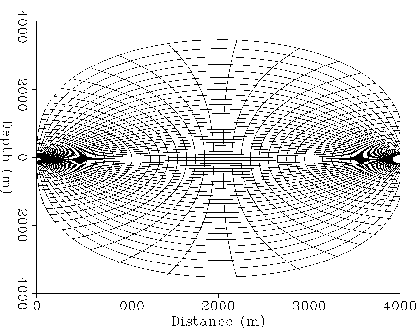

The potential field distribution nearby the singularities becomes nearly radially symmetric and mimics the shape of a wavefield emerging from a point source in a homogeneous medium. For simplicity, I force the initial extrapolation surface to be a circular arc that directly matches the point source wavefield. Although this introduces a slight non-orthogonality into an otherwise orthogonal mesh, this is taken into account by the RWE theory Shragge (2006a). In addition, I have situated the source point 50m below the free-surface in order to simulate ghost reflections commonly found in marine data. The forward modeled wavefield, $\Psi ({\bf s},{\bf r}; \omega)$, is thus generated by extracting from the wavefield the values at the receiver locations on the center line paralleling the free surface at the source depth.