

Next: Conclusions and Future Work
Up: Implementation of LSJIMP
Previous: SYN-1
hdata
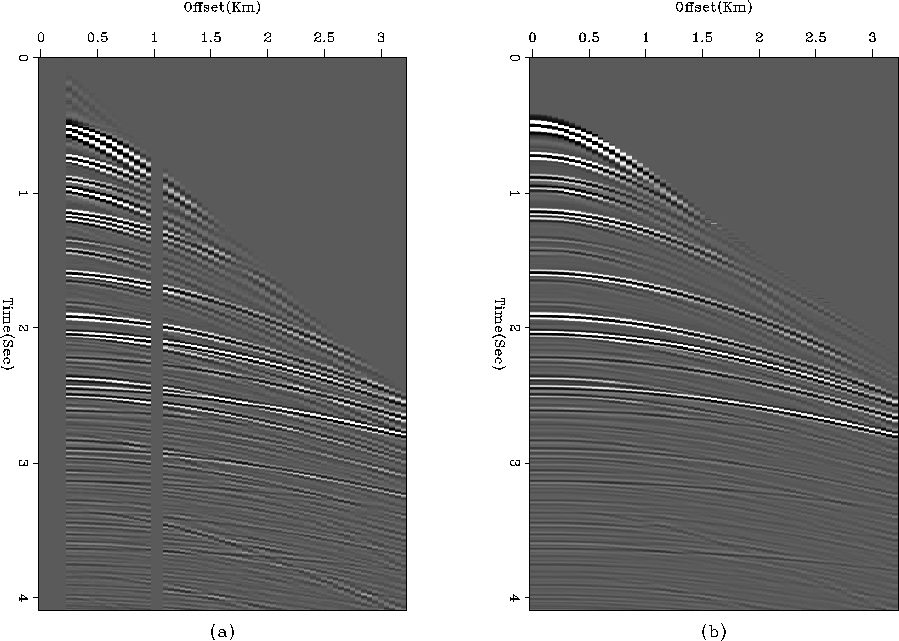
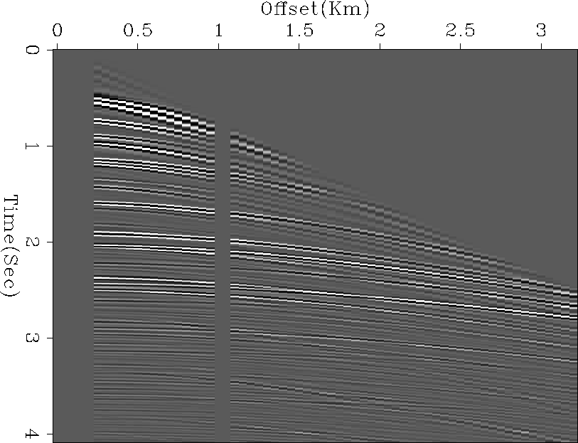
Figure 7 Hask Data Set


The "Hask" data set refers to Haskell-Thompson synthetic modeling. The dataset was modeled to resemble a North Sea data set donated by Mobil. We successfully apply LSJIMP to the Hask data set given in Figure ![[*]](http://sepwww.stanford.edu/latex2html/cross_ref_motif.gif) for imaging and suppressing the multiple energy. In Figure
for imaging and suppressing the multiple energy. In Figure ![[*]](http://sepwww.stanford.edu/latex2html/cross_ref_motif.gif) , we compare the raw data to the data generated by applying a forward modeling operator to our image, notice that much of the multiple energy is removed. Next, we compare our present result with results presented by Brown (2002) in Figure
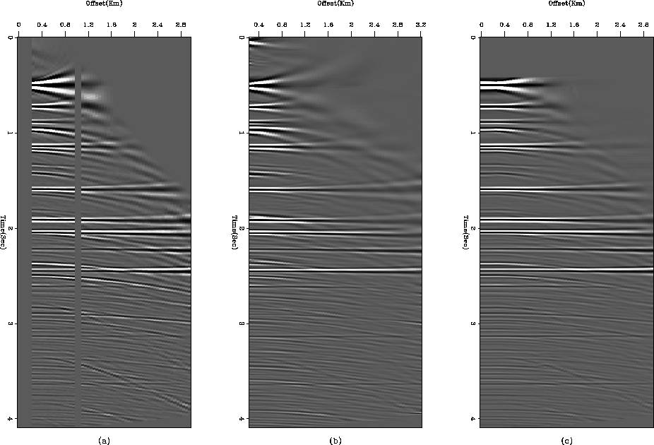
, we compare the raw data to the data generated by applying a forward modeling operator to our image, notice that much of the multiple energy is removed. Next, we compare our present result with results presented by Brown (2002) in Figure ![[*]](http://sepwww.stanford.edu/latex2html/cross_ref_motif.gif) . It can be observed that now we are doing a better job of multiple suppression in shallow parts. The primary reason being inclusion of crosstalk modeling operator in LSJIMP. The method used by Brown (2002) is equivalent to current method , with
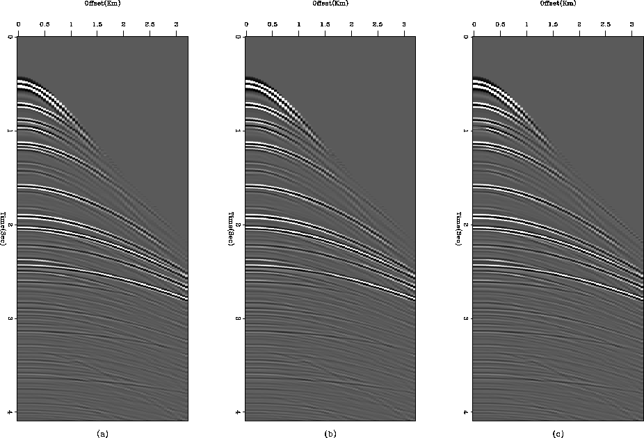
. It can be observed that now we are doing a better job of multiple suppression in shallow parts. The primary reason being inclusion of crosstalk modeling operator in LSJIMP. The method used by Brown (2002) is equivalent to current method , with  for crosstalk in equation (8) set equal to zero. To improve our performance on the Hask data set, we then took advantage of the fact that hask is also a shallow water-bottom data set and used the improved crosstalk-modeling strategy discussed in the previous section. Unfortunately, the results as given in Figure
 ![[*]](http://sepwww.stanford.edu/latex2html/cross_ref_motif.gif) do not seem to improve a lot.
do not seem to improve a lot.
We also tried a non-linear scheme Brown (2004) for updating reflection coefficients between two runs of LSJIMP. The presence of correlated events in the data residual ( ) hints at the likelihood for further improvements in estimates of the reflection coefficients. The main idea of the updating scheme is to compute a scalar update to the reflection coefficient of the
  multiple generator,
  , such that
|  |
(14) |
is minimized. We could not see any noticable difference with non-linear updates, as demonstrated in Figure ![[*]](http://sepwww.stanford.edu/latex2html/cross_ref_motif.gif) .
hask1
.
hask1
Figure 8 Comparison of (a) raw data and (b) results from first run of LSJIMP.


 hask-comp
Figure 9 Comparison of (a) raw data, (b) results presented in SEP-111 and (c) present results. Notice that a lot of multiple energy in the shallow parts is eliminated in our present results.


 hask2
hask2
Figure 10 Comparison of results from (a) LSJIMP, (b) LSJIMP(modified) and (c) LSJIMP after non-linear update.


Next: Conclusions and Future Work
Up: Implementation of LSJIMP
Previous: SYN-1
Stanford Exploration Project
4/5/2006

![[*]](http://sepwww.stanford.edu/latex2html/cross_ref_motif.gif) for imaging and suppressing the multiple energy. In Figure
for imaging and suppressing the multiple energy. In Figure ![[*]](http://sepwww.stanford.edu/latex2html/cross_ref_motif.gif) , we compare the raw data to the data generated by applying a forward modeling operator to our image, notice that much of the multiple energy is removed. Next, we compare our present result with results presented by Brown (2002) in Figure
, we compare the raw data to the data generated by applying a forward modeling operator to our image, notice that much of the multiple energy is removed. Next, we compare our present result with results presented by Brown (2002) in Figure ![[*]](http://sepwww.stanford.edu/latex2html/cross_ref_motif.gif) . It can be observed that now we are doing a better job of multiple suppression in shallow parts. The primary reason being inclusion of crosstalk modeling operator in LSJIMP. The method used by Brown (2002) is equivalent to current method , with
. It can be observed that now we are doing a better job of multiple suppression in shallow parts. The primary reason being inclusion of crosstalk modeling operator in LSJIMP. The method used by Brown (2002) is equivalent to current method , with ![]() for crosstalk in equation (8) set equal to zero. To improve our performance on the Hask data set, we then took advantage of the fact that hask is also a shallow water-bottom data set and used the improved crosstalk-modeling strategy discussed in the previous section. Unfortunately, the results as given in Figure
for crosstalk in equation (8) set equal to zero. To improve our performance on the Hask data set, we then took advantage of the fact that hask is also a shallow water-bottom data set and used the improved crosstalk-modeling strategy discussed in the previous section. Unfortunately, the results as given in Figure ![[*]](http://sepwww.stanford.edu/latex2html/cross_ref_motif.gif) do not seem to improve a lot.
do not seem to improve a lot.
![]() ) hints at the likelihood for further improvements in estimates of the reflection coefficients. The main idea of the updating scheme is to compute a scalar update to the reflection coefficient of the
) hints at the likelihood for further improvements in estimates of the reflection coefficients. The main idea of the updating scheme is to compute a scalar update to the reflection coefficient of the ![]() multiple generator,
multiple generator, ![]() , such that
, such that
![[*]](http://sepwww.stanford.edu/latex2html/cross_ref_motif.gif) .
.
