Theory

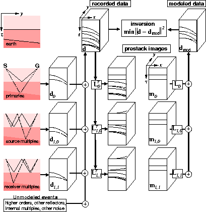
LSJIMP models the recorded data as the superposition of primary reflections and p orders of pegleg multiples from $n_{\rm surf}$ multiple-generating surfaces. A schematic for LSJIMP is given in Figure . An $i^{\rm th}$ order pegleg splits into i+1 legs. If we denote the primaries as $\bold d_0$ and the $k^{\rm th}$ leg of the $i^{\rm th}$ order pegleg from the $m^{\rm th}$ multiple generator as $\bold d_{i,k,m}$, the modeled data takes the following form:

 

schem-LSJIMP-seg
Figure 1 LSJIMP schematic. Assume that the recorded data consist of primaries and pegleg multiples. Prestack imaging alone (applying adjoint of modeling operator $\bold L_{i,k}$) focuses signal events in zero-offset traveltime (or depth) and offset (or reflection angle), but leaves behind crosstalk events. If the $\bold m_{i,k}$ images contain only signal, then we can model all the events in the data that we desire. The LSJIMP inversion suppresses crosstalk and endeavors to fit the recorded data in a least-squares sense. The model regularization operators used to suppress crosstalk simultaneously enable LSJIMP to exploit the intrinsic redundancy between and within the images to increase signal fidelity.

 

$$\bold d_{\rm mod} = \bold d_0 + \sum_{i=1}^p \sum_{k=0}^i \sum_{m=1}^{n_{\rm surf}} \bold d_{i,k,m}.$$ (1)

If we have designed an imaging operator that produces primary and multiple images with consistent signal (kinematics and angle-dependent amplitudes), then we assume that we can model the important events in the data. We can rewrite equation (1) as

$$\begin{eqnarray} \bold d_{\rm mod} &=& \bold L_0 \bold m_0 + \sum_{i=1}^p \sum_{... ...\rm surf}} \bold L_{i,k,m} \bold m_{i,k,m} \\ &=& \bold L \bold m\end{eqnarray}$$ (2) (3)

where $\bold L_0$ is the modeling operator of the primaries, and $\bold m_0$ is the image of primaries. Similarly, for the $k^{\rm th}$ leg of the $i^{\rm th}$ order pegleg from the $m^{\rm th}$ multiple generator, $\bold L_{i,k,m}$ and $\bold m_{i,k,m}$ are modeling operator and image respectively.

Brown (2004) derived appropriate imaging and amplitude correction operators to map the primary image, $\bold m_0$, into data-space primary events using the Normal Move-Out (NMO) operator, $\bold N_0$. Similarly, a given pegleg image, $\bold m_{i,k,m}$, is mapped into data space by sequentially applying the differential geometric spreading correction ($\bold G_{i,m}$), Snell resampling ($\bold S_{i,m}$), the Hetrogeneous-Earth Multiple NMO operator (HEMNO) ($\bold N_{i,k,m}$), and finally, a reflection coefficient ($\bold R_{i,k,m}$). HEMNO is a slight improvement over NMO that takes into account kinematics of mildly dipping reflectors. Using these operators, we can rewrite equation (2) as follows:  

$$\bold d_{\rm mod} = \bold N_0 \bold m_0 + \sum_{i=1}^p \sum... ...m} \bold N_{i,k,m} \bold S_{i,m} \bold G_{i,m} \bold m_{i,k,m}.$$ (4)

The LSJIMP seeks to optimize the primary and multiple images, $\bold m$,by minimizing the $\ell_2$ norm of the data residual, defined as the difference between the recorded data, $\bold d$, and the modeled data, $\bold d_{\rm mod}$[equation (3)]:  

$$\mbox{ \raisebox{-1.0ex}{ $\stackrel{\textstyle \mbox{min}}{... ...tyle \bold m} $} } \; \Vert \bold d - \bold L \bold m \Vert^2.$$ (5)

Minimization (5) is under-determined for many choices of prestack imaging operator, which implies an infinite number of least-squares-optimal solutions. The problem of infinite optimal solutions manifests itself as crosstalk leakage. Of this infinity of possible $\bf m$'s, we seek the one which not only fits the recorded data, but which also has minimum crosstalk leakage and maximum consistency between signal events on different images. In general we compensate for a correlated or poorly scaled data residual by adding a residual weighting operator, $\bf W_d$: 

$$\mbox{ \raisebox{-1.0ex}{ $\stackrel{\textstyle \mbox{min}}{... ...ert {\bf W_d} \left[ \bold d - \bold L \bold m \right] \Vert^2,$$ (6)

where strictly speaking,  

$$\left( {\bf W_d}^T {\bf W_d} \right)^{-1} = {\rm cov}[\bold d].$$ (7)

To effect the final step of LSJIMP and penalize crosstalk, we use three regularization operators. As discussed in detail by Brown (2004), the operators penalize roughness in reflection angle and between images, and also penalize the model after weighting with a prior model of the crosstalk on each $\bold m_{i,k,m}$. For estimation of the optimal set of $\bold m_{i,k,m}$, we minimize a quadratic objective function which consists of the sum of the weighted $\ell_2$ norms of the data residual [equation(6)] and of the three model residuals:  

$$\mbox{ \raisebox{-1.0ex}{ $\stackrel{\textstyle \mbox{min}}{... ...]} \Vert^2 \; + \; \epsilon_3^2 \Vert \bold r_m^{[3]} \Vert^2,$$ (8)

where $\epsilon_1, \epsilon_2,$ and $\epsilon_3$ are scalars that balance the relative weight of the three model residuals (damping factors) with the data residual. These three residuals are calculated by differencing across images, differencing across offset, generating a crosstalk model, and calculating their penalty weights.