


The data set was acquired in the Gulf of Mexico
over an existing reservoir.
Therefore several borehole seismic data sets
were available in addition to the surface data
to constraint the estimation of the anisotropic parameters.
ExxonMobil provided SEP with three anisotropic-parameter
cubes resulting from a joint inversion of the surface data
and the borehole data
Krebs et al. (2003).
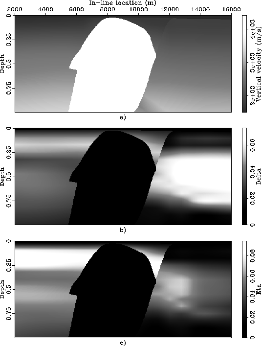
Figure ![[*]](http://sepwww.stanford.edu/latex2html/cross_ref_motif.gif) shows
the vertical slices cut through these cubes
at the cross-line location corresponding to the 2-D line
that I migrated.
Panel a) displays the vertical velocity,
panel b) displays the values of
shows
the vertical slices cut through these cubes
at the cross-line location corresponding to the 2-D line
that I migrated.
Panel a) displays the vertical velocity,
panel b) displays the values of ![]() ,and
panel c) displays the values of
,and
panel c) displays the values of ![]() .To avoid artifacts caused by sharp parameter contrasts,
for migration I removed the salt body from
the functions displayed in
Figure .
I ``infilled'' the salt body
with sediment-like values by interpolating
the functions inward starting from the sediment values
at the salt-sediment interface.
.To avoid artifacts caused by sharp parameter contrasts,
for migration I removed the salt body from
the functions displayed in
Figure .
I ``infilled'' the salt body
with sediment-like values by interpolating
the functions inward starting from the sediment values
at the salt-sediment interface.
 |
Figure
shows the result of anisotropic prestack depth migration.
All the reflectors are nicely imaged,
including the steep salt flank on the right-hand side of the salt body.
The shallow tract of the salt flank on the left-hand side of the body
is poorly imaged because it has large cross-line dip components.
The two vertical lines superimposed onto the image
identify the surface location of the ADCIGs displayed in
Figure .
The two black bars superimposed onto the image
identify the reflections for which I analyzed
the ADCIG in details.
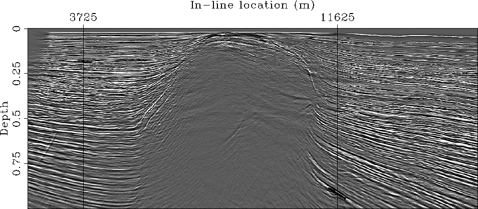 |
.
The two black bars superimposed onto the image
identify the reflections analyzed
in Figure .
|
Duo-aniso-overn
Figure 9 ADCIGs computed from the prestack image by slant stacking along the subsurface offset axis. The CIG shown in panel a) is taken at the surface location of 3,725 meters, and the CIG shown in panel b) is taken at the surface location of 11,625 meters. | 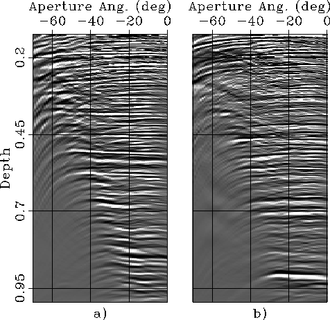 |


Figure shows two ADCIGs computed by slant stacking
the prestack image along the subsurface axis.
Both CIGs show fairly flat moveout,
indicating that the anisotropic velocity model used for migration is accurate,
though not perfect.
The shallow reflections show the most noticeable departure from flatness
(they frown downward) because these reflectors were not the focus of
the velocity model-building efforts.
The CIGs are taken at the location indicated by the vertical black lines
in Figure ; the CIG shown in panel a) is taken
at the surface location of 3,725 meters and the CIG shown in panel b) is taken
at the surface location of 11,625 meters.
Within these two CIGs, I selected for detailed analysis
the reflections corresponding to
the black bars superimposed onto the image
because they represent two `typical' cases
where the accuracy of the estimation of the reflection-aperture angle
might be important.
The shallow black bar on the left identifies a flat reflector illuminated with a wide
range of aperture angles, up to 60 degrees.
The wide angular range is potentially useful for constraining the
value of the anisotropic parameters in the sediments.
The deep black bar on the right identifies one of the potential reservoir
sands, and thus it is a potential target for Amplitude Versus Angle (AVA)
analysis using ADCIGs.
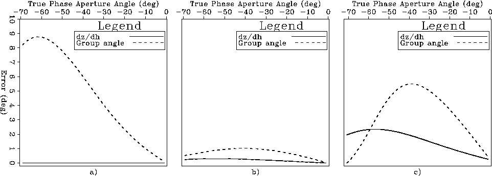
The plots in Figure show the differences
between the true phase aperture angle computed
by iteratively solving the system of equations 16 and 17
and the aperture angle estimated by slant stacks (solid line)
and the group aperture angle (dashed line).
The group angles are computed by applying equation 2.
The plot in panel a) corresponds
to the shallow black bar on the left.
The reflector is flat and the velocity parameters at the
reflector are:
![]() .As expected, the aperture angles estimated by slant stack are exactly the
same as the true ones because the reflector is flat.
The maximum difference between the group aperture angle and the phase aperture angle
is at 60 degrees, where the group angle is smaller
by about 9 degrees than the phase angle; that is, about an error of about 15%.
.As expected, the aperture angles estimated by slant stack are exactly the
same as the true ones because the reflector is flat.
The maximum difference between the group aperture angle and the phase aperture angle
is at 60 degrees, where the group angle is smaller
by about 9 degrees than the phase angle; that is, about an error of about 15%.
The plot in panel b) corresponds
the reservoir reflector (the deep black bar on the right).
The dip of the reflector is about 25 degrees and the velocity parameters
at the reflector are:
![]() .This area is weakly anisotropic (black in Figure b
in Figure c) and thus
the angular errors are small (
.This area is weakly anisotropic (black in Figure b
in Figure c) and thus
the angular errors are small (![]() 1 degree) even if the reflector
is dipping.
Finally, the plot in panel c) corresponds to the hypothetical situation in
which the reservoir was located in a more strongly anisotropic
area than it actually is.
To test the accuracy limits of approximating
the phase aperture angles with the subsurface-offset slopes in the prestack image,
I set the anisotropic parameters to be the highest value in the section;
that is:
1 degree) even if the reflector
is dipping.
Finally, the plot in panel c) corresponds to the hypothetical situation in
which the reservoir was located in a more strongly anisotropic
area than it actually is.
To test the accuracy limits of approximating
the phase aperture angles with the subsurface-offset slopes in the prestack image,
I set the anisotropic parameters to be the highest value in the section;
that is:
![]() ,and kept the vertical velocity and reflector's dip the same as
in the previous case.
The reflector is dipping and consequently the aperture angle
estimated by slant stacks is lower than the true aperture angle.
However, the error is small (
,and kept the vertical velocity and reflector's dip the same as
in the previous case.
The reflector is dipping and consequently the aperture angle
estimated by slant stacks is lower than the true aperture angle.
However, the error is small (![]() 2 degree) even at large
aperture angle,
and even smaller (
2 degree) even at large
aperture angle,
and even smaller (![]() 1 degree) within
the angular range actually illuminated
by the data (
1 degree) within
the angular range actually illuminated
by the data (![]() ).
Even in this ``extreme'' case the angular error
is unlikely to have any significant negative effect on the accuracy
of the AVA analysis of the reservoir reflection.
).
Even in this ``extreme'' case the angular error
is unlikely to have any significant negative effect on the accuracy
of the AVA analysis of the reservoir reflection.
 |
.
The plot in panel b) corresponds
the reservoir reflector (the deep black bar on the right).
The plot in panel c) corresponds to the hypothetical situation in
which the reservoir reflector was located in a more strongly anisotropic
area than it actually is.