Two Distinct Gassmann Materials, Uniform Fluid Saturation

This example and the next one will remove the restriction that the porous frame material is uniform. To have as much control as possible, we limit the heterogeneity to just two types of drained bulk moduli, K_d⁽¹⁾ and K_d⁽²⁾. These occur with a frequency measured by the volume fractions f₁ and f₂, respectively. These porous materials fill the space, so f₁ + f₂ = 1. The effective stress coefficient is known exactly for this model and is given by (20). This result is true both for homogeneously saturated two-component media (Berryman and Milton, 1991) as treated in this example, or for the type of patchy saturation treated in the next example. Proof of this statement is provided in Appendix A. For Gassmann's equations in each material, we also need either the fluid bulk modulus together with the layer porosities $\phi^{(1)}$ and $\phi^{(2)}$, or we just need the Skempton coefficient, B. For simplicity, we take B = 0.0 for uniform gas saturation, and B = 1.0 for uniform liquid saturation. (Although B = 1 may not be exactly correct for real liquid-saturated reservoirs, only the product $\alpha B$ is important for the modeling examples that follow. So desired differences in B can be introduced through differences in $\alpha$. In this way we hope to capture the essence of this problem using the minimum number of free parameters.) This summarizes the part of the modeling that is the same in this example and the next.

We will now assume that the fluid saturation is uniform throughout the stated model material: (1l,2l). [Notation indicates first layer is liquid filled (l) and second layer is also liquid filled. The alternative is that some layers are gas filled (g).]

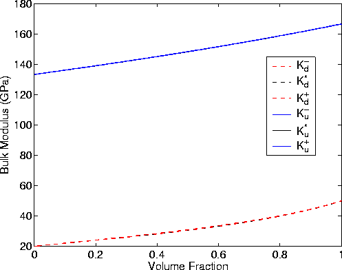
In Figure 6 there appear to be only two curves for bulk modulus, but in fact six curves are plotted here. All three of the drained curves are so close to each other that they cannot be distinguished on the scale of this plot. Similarly, all three of the undrained curves are equally indistinguishable.

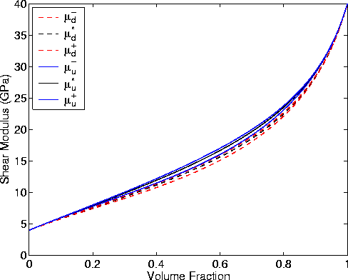
Figure 7 appears to be both qualitatively and quantitatively very similar to Figure 1. But this time we find the inequality $\mu_u^- \gt \mu_d^+$ is never violated. So there is no doubt that shear modulus is affected by pore fluids in this system.

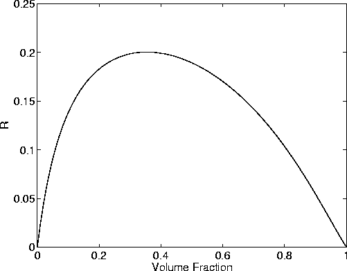
Figure 8 shows that the maximum value of $R \simeq 0.2$ occurs around $f_2 \simeq 0.3$. For this case, 4/15 is an upper bound on R, but I know this is not a general result.

 

Fig6
Figure 6 Illustrating the bulk modulus results for the random polycrystals of porous laminates model for homogeneous saturation when each grain is composed of two constituents: (1) K_d⁽¹⁾ = 20.0 GPa, $\mu_d^{(1)} = 4.0$ GPa and (2) K_d⁽²⁾ = 50.0 GPa, $\mu_d^{(2)} = 40.0$ GPa. Skempton's coefficient is taken to be B = 0.0 when the system is gas saturated, and B = 1.0 when the system is fully liquid saturated. The effective stress coefficients for the layers are, respectively, $\alpha^{(1)} = 0.85$ and $\alpha^{(2)} = 0.70$. Porosity does not play a direct role in the calculation when we are using B as the fluid substitution parameter. Volume fraction of the layers varies from 0 to 100% of constituent number 2.

 

Fig7
Figure 7 Illustrating the shear modulus results for the random polycrystals of porous laminates model. Model parameters are the same as in Figure 6 for homogeneous saturation.

 

Fig8
Figure 8 Plot of the ratio R from equation (24), being the ratio of compliance differences due to fluid saturation. These results are for the same model described in Figure 6 for homogeneous saturation. The values of R should be compared to those predicted by Mavko and Jizba (1991) for very low porosity and flat cracks, when $R = 4/15 \simeq 0.267$. We find in contrast that the random polycrystals of porous laminates model for the case considered always has $R \le 0.20$.