


Next: Estimation schemes based on
Up: CANONICAL FUNCTIONS AND THE
Previous: Canonical functions
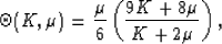
Some of the rigorous bounds that are expressible in terms of the
canonical functions for J = 2 are listed in TABLE 1. Functions and
averages required as definitions for some of the more complex terms in
TABLE 1 are:
|  |
(4) |
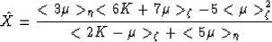
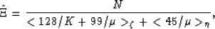
and the expressions needed for the McCoy-Silnutzer (MS) bounds
(McCoy, 1970; Silnutzer, 1972), which are
| ![\begin{displaymath}
\begin{array}
{rl}
X & = \left[10\mu_V^2\left<K\right\gt _\z...
...^2\left<\mu\right\gt _\eta\right]/(K_V+2\mu_V)^2,
\end{array} \end{displaymath}](img26.gif) |
(5) |
| ![\begin{displaymath}
\begin{array}
{rl}
\Xi & = \left[10K_V^2\left<K^{-1}\right\g...
...t<\mu^{-1}\right\gt _\eta\right]/(9K_V+8\mu_V)^2.
\end{array} \end{displaymath}](img27.gif) |
(6) |
The averages 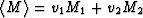 ,
,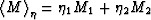 , and
, and
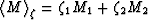 are defined for any
modulus M.
The volume fractions are v1,v2, while
are defined for any
modulus M.
The volume fractions are v1,v2, while  and
and
 are the microgeometry parameters or
Milton numbers (Milton, 1981; 1982), related to spatial correlation functions of the composite
microstructure. The Voigt averages of the moduli are
are the microgeometry parameters or
Milton numbers (Milton, 1981; 1982), related to spatial correlation functions of the composite
microstructure. The Voigt averages of the moduli are
 and
and  .For symmetric cell materials:
  for spherical
cells,
for spherical
cells,  for disks, while
 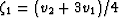 and
and 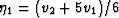 for needles.
Alternative bounds that are at least as tight as the
McCoy-Silnutzer (MS) bounds for any choice
of microstructure were given by Milton and Phan-Thien (1982)
as
|  |
(7) |
and
|  |
(8) |
where
|  |
(9) |
It has been shown numerically that the two sets of bounds
(MS and MPT) using the transform parameters
X, and
and  ,
, are nearly indistiguishable
for the penetrable sphere model (Berryman, 1985).
are nearly indistiguishable
for the penetrable sphere model (Berryman, 1985).
Note that ``improved bounds'' are not necessarily improved
for every choice of volume fraction, constituent moduli, and
microgeometry. It is possible in some cases that
``improved bounds'' will actually be less restrictive, than say
the Hashin-Shtrikman bounds, for some range of the parameters. In
such cases we obviously prefer to use the more restrictive bounds
when our parameters happen to fall in this range.
Milton (1987; 2002) has shown that, for the commonly
discussed case of two-component composites, the canonical functionals
can be viewed as fractional linear transforms with the arguments
 and
and  of the canonical functionals as the transform
variables. In light of the monotonicity properties of the functionals,
this point of view is very useful because the problem of determining
estimates of the moduli can then be reduced to that of finding
estimates of the parameters and . Furthermore,
properties of the canonical functions also imply that excellent
estimates of the moduli can be obtained from fairly crude estimates of the
transformation parameters and . (Recall, for example,
that estimates of zero and infinity for these parameters result in
Reuss and Voigt bounds on the moduli.) Milton calls this
transformation procedure the Y-transform, where Y stands for one
of these transform parameters (i.e., and in
elasticity, or another combination when electrical conductivity
and/or other mathematically analogous properties are being
considered).
of the canonical functionals as the transform
variables. In light of the monotonicity properties of the functionals,
this point of view is very useful because the problem of determining
estimates of the moduli can then be reduced to that of finding
estimates of the parameters and . Furthermore,
properties of the canonical functions also imply that excellent
estimates of the moduli can be obtained from fairly crude estimates of the
transformation parameters and . (Recall, for example,
that estimates of zero and infinity for these parameters result in
Reuss and Voigt bounds on the moduli.) Milton calls this
transformation procedure the Y-transform, where Y stands for one
of these transform parameters (i.e., and in
elasticity, or another combination when electrical conductivity
and/or other mathematically analogous properties are being
considered).
Next: Estimation schemes based on
Up: CANONICAL FUNCTIONS AND THE
Previous: Canonical functions
Stanford Exploration Project
5/3/2005