| |
(1) |
The minimum of ![]() can be found by solving the generalized eigensystem:
can be found by solving the generalized eigensystem:
| |
(2) |
For application to seismic salt interfaces, we merely apply the algorithm to instantaneous amplitude. Several cost saving techniques are explored in Lomask et al. (2004).
By applying bounds we greatly reduce the size of the problem. These initial rough bounds can be found by first running the algorithm with small search neighborhoods and coarse sampling.
|
pic2
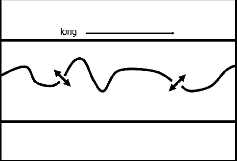
Figure 1 A cartoon of a masked salt boundary. It is long and thin with a discontinuous salt boundary snaking across it. |  |
Unfortunately, the normalized cut segmentation method tends to partition elongated images along their shortest dimension. For instance, Figure ![[*]](http://sepwww.stanford.edu/latex2html/cross_ref_motif.gif) is a cartoon of an elongated image with a salt boundary snaking across it. If the segmentation algorithm were to function as hoped, the minimum cut would be found along the salt boundary. However, because the salt boundary is discontinuous, it is likely that the minimum of the normalized cut in equation (1) will be found by cutting the image vertically where the image is thin.
is a cartoon of an elongated image with a salt boundary snaking across it. If the segmentation algorithm were to function as hoped, the minimum cut would be found along the salt boundary. However, because the salt boundary is discontinuous, it is likely that the minimum of the normalized cut in equation (1) will be found by cutting the image vertically where the image is thin.
To correct this problem, we exploit the fact that the upper boundary will necessarily be in Group A and the lower boundary will be in Group B. In other words, we want to force the segmentation algorithm to put the coarsely picked bounds in different groups.
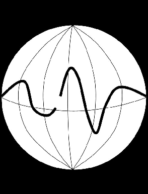
We can enforce this constraint during the creation of the weight matrix (![]() ). Recall that this matrix contains weights relating each sample to every other sample along paths within a neighborhood. For any given sample, if its search neighborhood happens to cross a coarse boundary, it becomes weighted to every other sample near the boundary. This can be imagined by wrapping the image on a globe so that both the upper and lower bounds collapse to points at the poles (see Figure
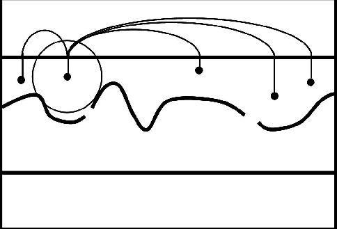
). Recall that this matrix contains weights relating each sample to every other sample along paths within a neighborhood. For any given sample, if its search neighborhood happens to cross a coarse boundary, it becomes weighted to every other sample near the boundary. This can be imagined by wrapping the image on a globe so that both the upper and lower bounds collapse to points at the poles (see Figure ![[*]](http://sepwww.stanford.edu/latex2html/cross_ref_motif.gif) ). When estimating the weight matrix, every time a path crosses the north or south pole, it continues down the other side. In Cartesian space, this can be seen in the cartoon in Figure
). When estimating the weight matrix, every time a path crosses the north or south pole, it continues down the other side. In Cartesian space, this can be seen in the cartoon in Figure ![[*]](http://sepwww.stanford.edu/latex2html/cross_ref_motif.gif) .
.
|
pic6
Figure 2 A cartoon illustrating global bounds. The image is stretched onto a sphere and the upper and lower boundaries of the mask collapse to points. |  |
|
pic5
Figure 3 A cartoon illustrating idealized global bounds. When the search area for a node reaches outside the mask (as shown by the circle on the left), it becomes connected to all points along the boundary. |  |
This ``Global'' bounds approach is completely impractical because it creates as many new weights as are saved by the size reduction of the problem.
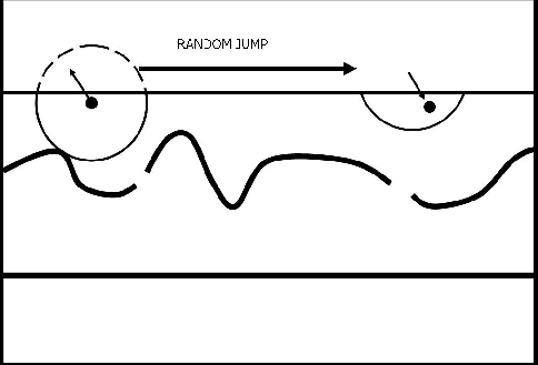
A more practical approach that is still essentially the same concept is ``Random'' bounds. This is illustrated in Figure ![[*]](http://sepwww.stanford.edu/latex2html/cross_ref_motif.gif) . Every time a path crosses a bound, it jumps a random distance along the boundary.
. Every time a path crosses a bound, it jumps a random distance along the boundary.
|
pic4
Figure 4 A cartoon illustrating the more practical random bounds. When the search area for a node reaches outside the mask (as shown by the circle on the left), it is connected to a single node a random distance along the boundary. |  |
We have implemented and tested this random bounds method and found that it works well in our preliminary test cases.