


Next: Numerical Examples
Up: Theory
Previous: Generating Potential Functions
The next processing step involves tracing geometric coordinate system
rays from the generated PF. The goal here is
to develop an orthogonal, ray-based coordinate system related to an
underlying Cartesian mesh through one-to-one mappings,
| 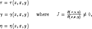 |
|
| (7) |
| |
where  is the wavefield extrapolation direction (equivalent
to z in Cartesian),
is the wavefield extrapolation direction (equivalent
to z in Cartesian),  and
and  are the two orthogonal
directions (equivalent to x and y in Cartesian), and J is the
Jacobian of the coordinate system transformation. Recorded wavefield,
are the two orthogonal
directions (equivalent to x and y in Cartesian), and J is the
Jacobian of the coordinate system transformation. Recorded wavefield,
 , is extrapolated from the acquisition surface
defined by
, is extrapolated from the acquisition surface
defined by  into the subsurface along the rays coordinate system
defined by triplet
into the subsurface along the rays coordinate system
defined by triplet ![$\left[\tau,\gamma,\eta\right]$](img33.gif) .
.
Geometric rays are traced by solving a first-order ordinary
differential equation through integrating the PF gradient field
along the gradient direction,
| ![\begin{displaymath}
\delta \phi = \int_{a(z_0,x_0,y_0)}^{b(z_1,x_1,y_1)} \vert...
...tial x}+ {\rm d}y \frac{\partial \phi} {\partial y}
\right],
\end{displaymath}](img34.gif) |
(8) |
where a(z0,x0,y0) is a known lower integration bound at
equipotential  , and b(z1,x1,y1) is an unknown upper
integration bound located on equipotential surface,
, and b(z1,x1,y1) is an unknown upper
integration bound located on equipotential surface,  , and
, and
 is the L2 norm of the gradient function.
The only unknown parameter is b(z1,x1,y1);
hence, Equation (8) is an integral equation with an
unknown integration bound. This approach is similar to phase-ray
tracing method described in Shragge and Sava (2004b); however,
in this case the integration step lengths are now unknown. Note also
that the equipotentials of the upper and lower bounding surfaces in
Equation (4) require PF steps of
is the L2 norm of the gradient function.
The only unknown parameter is b(z1,x1,y1);
hence, Equation (8) is an integral equation with an
unknown integration bound. This approach is similar to phase-ray
tracing method described in Shragge and Sava (2004b); however,
in this case the integration step lengths are now unknown. Note also
that the equipotentials of the upper and lower bounding surfaces in
Equation (4) require PF steps of  .
.
The following approach locates unknown integration bound, b, on the
next equipotential:
- 1.
- Numerically integrate Equation (8) on the interval
[
 ] where
  is smaller than the expected step
size, and test to see whether
is smaller than the expected step
size, and test to see whether 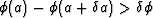 ; if yes goto step 3;
- 2.
- Numerically integrate Equation (8) on next interval
![$[a+\delta a,a+2\delta a]$](img42.gif) and test whether
and test whether  ; if yes goto step 3; if no, repeat step 2 n
times until true;
; if yes goto step 3; if no, repeat step 2 n
times until true;
- 3.
- Linearly interpolate between points
 and
and
 to find the b corresponding to
 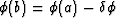 .
.
A geometric ray is initiated at a particular ![$[\gamma_0, \eta_0]$](img47.gif) on acquisition surface defined by , and computed by
integrating through each successive
on acquisition surface defined by , and computed by
integrating through each successive  step until the lower
bounding surface
step until the lower
bounding surface  is reached. This procedure is repeated for
all and acquisition points.
is reached. This procedure is repeated for
all and acquisition points.
Next: Numerical Examples
Up: Theory
Previous: Generating Potential Functions
Stanford Exploration Project
5/3/2005