methodology

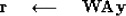
Equation (1) is taken from Chapter 6. of Claerbout (1999).  

$$\bold 0 \quad\approx\quad \left[ \begin{array} {cc} \bol... ...y \\ \Delta \bold a \end{array} \right] \ +\ \bar {\bold r}.$$ (1)

This fitting goal estimates both missing data and a filter simultaneously. $\bold A$ and $\bold Y$ are the convolutional matrix algebraic notations for the filter and the data, respectively. $\bold{\Delta a}$ and $\bold{\Delta y}$ are perturbation vectors for the filter and the data. The free-mask matrix for missing data is denoted $\bold J$ and that for the PEF is $\bold K$. The original residual is defined as $\bar {\bold r} = \bold A\bold y$.

Next, a diagonal weight matrix $\bold W$ can be applied to the residual as:  

$$\bold 0 \quad\approx\quad \bold W \left[ \left[ \begin{ar... ...ta \bold a \end{array} \right] \ +\ \bar {\bold r} \right] .$$ (2)

This weight is used to remove any fitting equations in which the filter has fewer than a specified number of coefficients on known data. The number of coefficients that are on known data at each point in the model can be thought of as the coefficient fold. The range of coefficient fold values is broken up into several steps. Equation (2) is first solved using fitting equations with coefficient fold greater than the highest step. Then the resulting PEF and missing data are used as the initial solution for the next step. This is repeated and the 2D PEF is gradually built up.

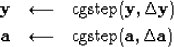
Within the solver, the following equations are iterated over Claerbout (1999):  

$$\bold r \quad\longleftarrow\quad \bold {WAy}$$ (3)

 

$$\left[ \begin{array} {c} \Delta \bold y \\ \Delta \bold a... ...d A' \\ \bold K' \bold Y' \end{array} \right] \ \bold {W'r}$$ (4)

 

$$\Delta \bold r \quad\longleftarrow\quad \bold W \left[ \b... ...ay} {c} \Delta \bold y \\ \Delta \bold a \end{array} \right]$$ (5)

$$\begin{eqnarray} \bold y &\longleftarrow& {\rm cgstep}( \bold y, \Delta \bold y) \\ \bold a &\longleftarrow& {\rm cgstep}( \bold a, \Delta \bold a)\end{eqnarray}$$ (6) (7)

 

• Balancing the unknown data and the filter