


WesternGeco supplied a depth interval velocity model with the data. I migrated the raw data and the LSJIMP primary data using a 2-D Extended Split-Step prestack depth migration algorithm Stoffa et al. (1990) with three so-called ``reference velocities'' to handle lateral velocity variation. Image sampling in depth is 6.67 meters. The migration algorithm outputs gathers as a function of depth, midpoint, and subsurface offset. Using the method of Sava and Fomel (2000), the offset gathers are converted to Angle-domain Common-image gathers (ADCIGs) as a function of opening angle at the reflector.
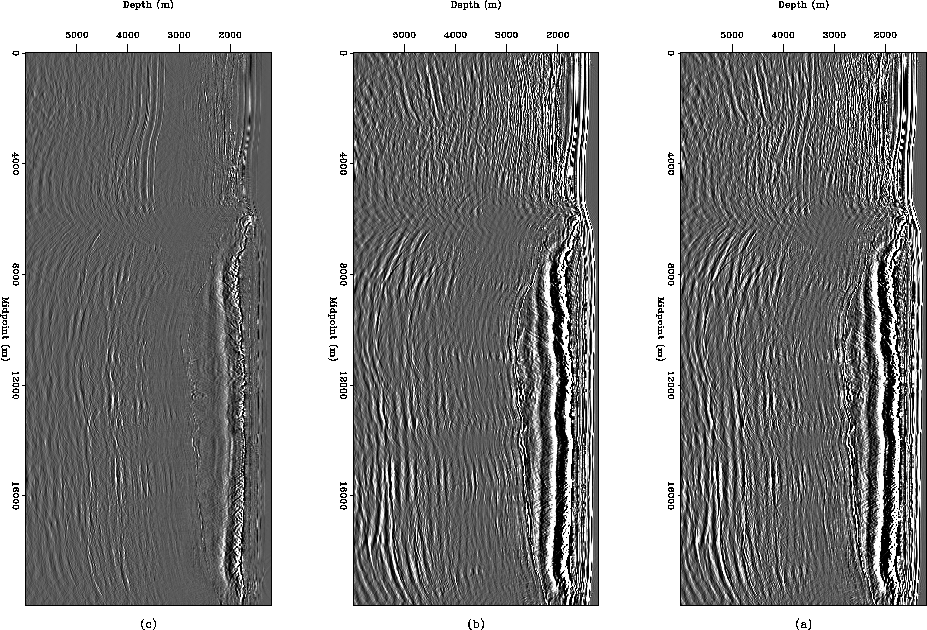
Figure ![[*]](http://sepwww.stanford.edu/latex2html/cross_ref_motif.gif) shows angle stacks, after a z1.5
gain, of the Mississippi Canyon raw data, the data after LSJIMP, and the
difference of the two. The Figure is similar in style to Figure
. The removed multiples are simplest to view on the
left-hand side of the section, where the geology is less complicated than under
the salt body. In the sedimentary region, we notice, as before, that LSJIMP can
cleanly separate primaries from many different multiple reflections. In the
salt region, the results are somewhat muddied, since migration strongly
defocuses multiples. We see that much multiple energy has been removed, though
much remains. Subsalt primaries, already difficult to spot without any multiple
energy, are uncovered better, especially around 3500 meters depth. The dominant
dip is negative (toward the surface with increasing midpoint).
shows angle stacks, after a z1.5
gain, of the Mississippi Canyon raw data, the data after LSJIMP, and the
difference of the two. The Figure is similar in style to Figure
. The removed multiples are simplest to view on the
left-hand side of the section, where the geology is less complicated than under
the salt body. In the sedimentary region, we notice, as before, that LSJIMP can
cleanly separate primaries from many different multiple reflections. In the
salt region, the results are somewhat muddied, since migration strongly
defocuses multiples. We see that much multiple energy has been removed, though
much remains. Subsalt primaries, already difficult to spot without any multiple
energy, are uncovered better, especially around 3500 meters depth. The dominant
dip is negative (toward the surface with increasing midpoint).
For reasons explained in more detail in section , some
primary energy is seen on the difference panel, where we hope to see only
multiple energy. The loss of primary energy, while well below the clip value
anywhere, is strongest for the top of salt reflection. Much of the lost energy
has a high spatial wavenumber, and likely arises from diffractions which my
implementation of LSJIMP cannot model. Also, the large velocity contrast at the
top of salt gives rise to strong head waves, which have a high apparent velocity.
These events, which are not flat after NMO for primaries, are filtered out as
noise by the LSJIMP regularization which differences across offset.
 |
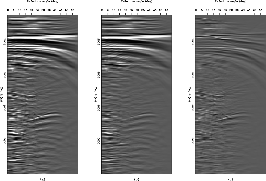
Figures and
illustrate, after z1.5 gain, ADCIGs at midpoints 55 and 344 (of 750),
respectively. Compare these Figures to Figures
and . Figure is
extracted from the sedimentary region of the data. Notice that LSJIMP has quite
cleanly separated multiples from the primaries, and certainly improved our
ability to interpret the angle gather for amplitude-versus-angle phenomena.
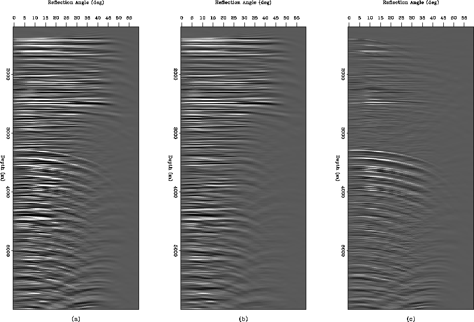 |
Figure , on the other hand, is extracted from
the salt-bearing region of the data. Visually, it is far more difficult on the
angle gather to distinguish primaries from multiples, although peglegs from
shallow reflectors, between 3500 and 4300 meters depth, are recognizable and
cleanly removed from the data, uncovering some hidden primaries. Notice that
some downcurving reflections within the salt (1900 to 2800 meters depth), which
may be internal multiples, are attenuated by LSJIMP, since they are not flat like
true signal events. Furthermore, the events with negative dip below 4000 meters,
which may be out-of-plane reflections or diffractions, are also attenuated
somewhat.
 |
![[*]](http://sepwww.stanford.edu/latex2html/movie.gif)


