Finite-difference solution to the $15^\circ$ equation

This appendix details the computations associated with the finite-difference solution to the $15^\circ$ equation in a 2-D orthogonal Riemannian space.

The 3-D wave equation (22) takes in two dimensions the simpler form:

$$k_\zeta\approx i \frac{\c_{\zeta}}{2\c_{\zeta\zeta}} + \; k_... ...right)^2-\frac{\c_{\xi\xi}}{\c_{\zeta\zeta}} \right]k_\xi^2 \;.$$ (38)

If we substitute the Fourier-domain wavenumbers by their equivalent space-domain partial derivatives, we obtain  

$$\frac{\partial \mathcal{U}}{\partial k_\zeta } \approx -\fra... ...ta}} \right]\frac{\partial^2 \mathcal{U}}{\partial k_\xi^2} \;.$$ (39)

A finite-difference implementation of equation (39) involving the Crank-Nicolson method is

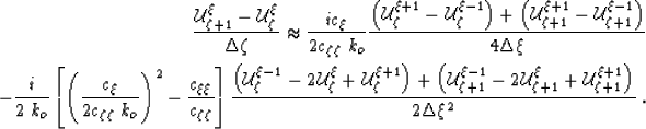$$\begin{eqnarray} \frac{\mathcal{U}^{\xi} _{\zeta+1}-\mathcal{U}^{\xi} _{\zeta}}{... ..._{\zeta+1}+\mathcal{U}^{\xi+1}_{\zeta+1}\right)}{2\Delta\xi^2} \;.\end{eqnarray}$$ (40)

If we make the notations

$$\begin{eqnarray} \mu &=& \frac{i\c_{\xi}}{2\c_{\zeta\zeta}\; k_o} \frac{\Delta\... ...xi}}{\c_{\zeta\zeta}} \right] \frac{\Delta\zeta}{2\Delta\xi^2} \;,\end{eqnarray}$$ (41)

we can write equation (40) as

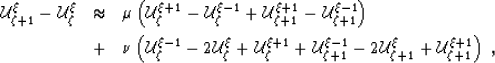$$\begin{eqnarray} \mathcal{U}^{\xi} _{\zeta+1}-\mathcal{U}^{\xi} _{\zeta}&\approx... ...athcal{U}^{\xi} _{\zeta+1}+\mathcal{U}^{\xi+1}_{\zeta+1}\right)\;,\end{eqnarray}$$ (42)

or, if we isolate the terms corresponding to the two extrapolation levels as:

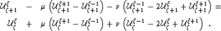$$\begin{eqnarray} \mathcal{U}^{\xi} _{\zeta+1}&-& \mu \left(\mathcal{U}^{\xi+1}_{... ...-2\mathcal{U}^{\xi} _{\zeta}+\mathcal{U}^{\xi+1}_{\zeta}\right)\;.\end{eqnarray}$$ (43)

After grouping the terms, we obtain

$$-\left(\nu-\mu \right)\mathcal{U}^{\xi-1}_{\zeta+1}+ \left(1... ...i} _{\zeta}+ \left(\nu+\mu\right)\mathcal{U}^{\xi+1}_{\zeta}\;,$$

which is a finite-difference representation of the $15^\circ$ solvable using fast tridiagonal solvers.