DISPERSION RELATIONS FOR SEISMIC WAVES

The general behavior of seismic waves in anisotropic media is well known, and the equations are derived in many places including Berryman (1979) and Thomsen (1986). The results are

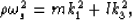
$$\begin{eqnarray} \rho\omega_{\pm}^2 = {{1}\over{2}} \left\{(a+l)k_1^2 + (c+l)k_3... ...\sqrt{[(a-l)k_1^2 - (c-l)k_3^2]^2 + 4(f+l)^2k_1^2k_3^2}\right\}, \end{eqnarray}$$ (35)

for compressional (+) and vertically polarized shear (-) waves and

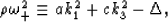
$$\begin{eqnarray} \rho \omega_s^2 = mk_1^2 + lk_3^2, \end{eqnarray}$$ (36)

for horizontally polarized shear waves, where $\rho$ is the overall density, $\omega$ is the angular frequency, k₁ and k₃ are the horizontal and vertical wavenumbers (respectively), and the velocities are given simply by $v = \omega/k$ with $k = \sqrt{k_1^2 + k_3^2}$. The SH wave depends only on elastic parameters l and m, which are not dependent in any way on layer $\lambda$ and therefore will play no role in the poroelastic analysis. Thus, we can safely ignore SH except when we want to check for shear wave splitting (bi-refringence) - in which case the SH results will be useful for the comparisons.

The dispersion relations for quasi-P- and quasi-SV-waves can be rewritten in a number of instructive ways. One of these that we will choose for reasons that will become apparent shortly is

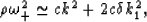
$$\begin{eqnarray} \rho\omega_{\pm}^2 = {{1}\over{2}} \left[(a+l)k_1^2 + (c+l)k_3^... ...(ak_1^2+ck_3^2)lk^2 + \{(a-l)(c-l)-(f+l)^2\}k_1^2k_3^2]}\right]. \end{eqnarray}$$ (37)

Written this way, it is then obvious that the following two relations hold:

$$\begin{eqnarray} \rho\omega_{+}^2 + \rho\omega_{-}^2 = (a+l)k_1^2 + (c+l)k_3^2, \end{eqnarray}$$ (38)

and

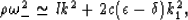
$$\begin{eqnarray} \rho\omega_{+}^2\cdot\rho\omega_{-}^2 = (ak_1^2+ck_3^2)lk^2 + [(a-l)(c-l)-(f+l)^2]k_1^2k_3^2, \end{eqnarray}$$ (39)

either of which could have been obtained directly from (35) without the intermediate step of (37).

We are motivated to write the equations in this way in order to try to avoid evaluating the square root in (35) directly. Rather, we would like to arrive at a natural approximation that is quite accurate, but does not involve the square root operation. From a general understanding of the problem, it is clear that a reasonable way of making use of (38) is to make the identifications

$$\begin{eqnarray} \rho\omega_{+}^2 \equiv ak_1^2 + ck_3^2 - \Delta, \end{eqnarray}$$ (40)

and

$$\begin{eqnarray} \rho\omega_{-}^2 \equiv lk^2 + \Delta, \end{eqnarray}$$ (41)

with $\Delta$ still to be determined. Then, substituting these expressions into (39), we find that

$$\begin{eqnarray} (ak_1^2 + ck_3^2 - lk^2 - \Delta)\Delta = [(a-l)(c-l)-(f+l)^2]k_1^2k_3^2 \end{eqnarray}$$ (42)

Solving (42) for $\Delta$ would just give the original results back again. So the point of (42) is not to solve it exactly, but rather to use it as the basis of an approximation scheme. If $\Delta$ is small, then we can presumably neglect it inside the parenthesis on the left hand side of (42), or we could just keep a small number of terms in an expansion.

The leading term, and the only one we will consider here, is

$$\begin{eqnarray} \Delta = {{[(a-l)(c-l)-(f+l)^2]k_1^2k_3^2}\over {(a-l)k_1^2 + (... ...simeq {{[(a-l)(c-l)-(f+l)^2]}\over {(a-l)/k_3^2 + (c-l)/k_1^2}}. \end{eqnarray}$$ (43)

The numerator of this expression is known to be a positive quantity for layered materials (Postma, 1955; Berryman, 1979). Furthermore, it can be rewritten in terms of Thomsen's parameters as

$$\begin{eqnarray}[(a-l)(c-l)-(f+l)^2] = 2c(c-l)(\epsilon-\delta). \end{eqnarray}$$ (44)

Using the first of the identities noted earlier in (5), we can also rewrite the first elasticity factor in the denominator as $a-l = (c-l)[1+2c\epsilon/(c-l)]$. Combining these results in the limit of $k_1^2 \to 0$ (for relatively small horizontal offset), we find that

$$\begin{eqnarray} \rho\omega_{+}^2 \simeq ck^2 + 2c\delta k_1^2, \end{eqnarray}$$ (45)

and

$$\begin{eqnarray} \rho\omega_{-}^2 \simeq lk^2 + 2c(\epsilon-\delta)k_1^2, \end{eqnarray}$$ (46)

with $\Delta \simeq 2c(\epsilon-\delta)k_1^2$.Improved approximations to any desired order can be obtained with only a little more effort by using (42) or (43) instead of the first approximation used here. But (45) and (46) are satisfactory for our present purposes.